2026-05-16. The 2025 Sidhom dual-attention LLM for somatic mutations hooked me on the architecture, not the biology. The same recipe keeps showing up across problems that look nothing alike — amino acids, mutation contexts, cell morphologies — running through the same stack with just the input alphabet swapped. If it’s already substrate-independent across biology, is materials science the next substrate? That’s the bet this note works out.
Background
A lot of scientific predictions are bag-of-things → sample-label: a patient and their thirty-odd somatic mutations; a biopsy slide and a million patches; a doped catalyst and a list of defect sites. The label is on the whole thing; the data is a bag; you don’t know up front which item drove it. This is multiple-instance learning. The classic hand-craft-and-pool recipe throws away the question scientists actually want answered: which item drove the prediction.
Ilse, Tomczak & Welling (ICML 2018) published the modern fix: an attention pool that learns a weight for each item end-to-end and combines them as a weighted sum. Per-item features are learned, not engineered; the weights are the interpretability output; training is one graph. Whether attention is strictly more faithful than gradient attributions is a live debate (Jain & Wallace 2019); the practical point is the interpretability map falls out of the architecture for free, and a causal-perturbation test (AOPC, §6) can validate it post-hoc.
Pathology picked it up first (CLAM, TransMIL), then immunology (DeepTCR), then oncology (ATGC, then the 2025 Sidhom LLM). Each time the attention map was scientifically usable. The NLP half of the recipe — discrete vocabulary, learnable embeddings, masked-token pretrain, fine-tune — moved through biology one alphabet at a time (proteins via ProtBERT/ESM, DNA via DNABERT, TCRs via DeepTCR, mutations via the Sidhom LLM). Materials science is the next alphabet to try.
Figure 2. The “biology-as-language” research program in one picture. Every row uses the same architecture on the right; only the discrete vocabulary on the left changes. The last row — defects in a doped crystal — is the bet this note is testing.
Sidhom’s framing for the biological line is “the language of cancer.” Mutation = word, tumor = document, co-occurring mutations = syntax, with a sentence-then-document attention hierarchy (local attention over DNA context around each mutation, then global attention over the bag of mutations). Documents have order, mutation bags don’t, which is why the permutation-invariant MIL aggregator — not the transformer — is the load-bearing piece. The materials port is the same move once more: vocabulary becomes defect sites / Wyckoff sites / monomers, “sentence” becomes the local coordination shell, and the sample is a bag of those.
1. The methodology, in domain-neutral form
Figure 3. The recipe in pipeline form. Top labels are the primitives; bottom labels are what each one resolves to in immunology / oncology / materials (the three substrates discussed below).
Five primitives, each load-bearing:
- Trainable token embedding from scratch. Pick a discrete unit (amino acid, mutation, dopant species). Give it a learnable vector. Let context teach the model what it means. No hand-crafted descriptors.
- Variable-length per-instance backbone. Each instance is a short variable-length sequence — CDR3, mutation context, defect coordination shell. CNN works (DeepTCR), Transformer works (the 2025 LLM). The backbone returns one dense vector per instance.
- Side-information / metadata channel. Categorical context that isn’t part of the sequence itself — V/D/J gene, MHC allele, tissue of origin — is embedded separately and fused with the sequence representation. The materials analog is space group, lattice type, synthesis route, processing history.
- Two-level attention.
- Local (sequence-aware) attention: order-sensitive, captures what the token means in immediate context.
- Global (permutation-invariant) attention: aggregates instances across the sample, captures co-occurrence without imposing a spurious order.
- Attention-based multiple-instance learning (MIL). Labels live at the sample level (patient outcome, tumor type, immunotherapy response). The model must aggregate a bag of per-instance vectors into a single sample-level prediction with per-instance importance weights you can read off. This is the part most people don’t import from NLP, and it is what turns “model that embeds one mutation” into “model that diagnoses a tumor.”
Bonus, used heavily in the 2025 model: MAE-style masked-token pretraining (literally 100% masking on the altered sequence) before the supervised head. Lines up with the TempoSurfViT recipe already in our toolkit (MAE pretrain + quantile head, paper draft at /writing/temposurfvit-draft/), so very little engineering overhead.
Equivariance: the materials-specific commitment
SO(3) rotational symmetry is the hard problem the bio version doesn’t have to face — amino-acid sequences are already 1-D, mutation contexts are already textual, but a defect site lives in 3-D space whose labelling is gauge-arbitrary. Three families of published options:
- Scalar invariants (SOAP, ACE). Pre-computed rotation-invariant descriptors. Cheap, well-tested on small molecules, but throw away geometric structure the network might want.
- Equivariant message passing (NequIP, MACE). SO(3) preserved end- to-end, strong on potential-energy surfaces, but the bag pool we want to put on top is permutation-symmetric, not rotation- equivariant — composing the two needs care.
- Equivariant transformer (EquiformerV2 / UMA). What the strongest
2026 catalyst baselines use. EquiformerV2-OC22 checkpoints are no
longer publicly downloadable from Meta; UMA-s-1p2 is the official
fairchem 2.x successor — same lab, multi-task pretrained including
OC22, ~2.2 GB checkpoint, public on HuggingFace under
facebook/UMA. This is what we actually use.
The cleanest commit for v1: frozen UMA-s-1p2 as the per-instance backbone, applied to a local cluster centered on each site, pooled within the cluster to one -dim SO(3)-invariant vector before entering the bag. Equivariance is enforced at the per-instance level; the MIL pool acts on already-invariant vectors and inherits invariance trivially. The cost is compute (no MPS acceleration; cloud GPU for training); the win is that we don’t reinvent equivariant representation learning in the aggregator itself.
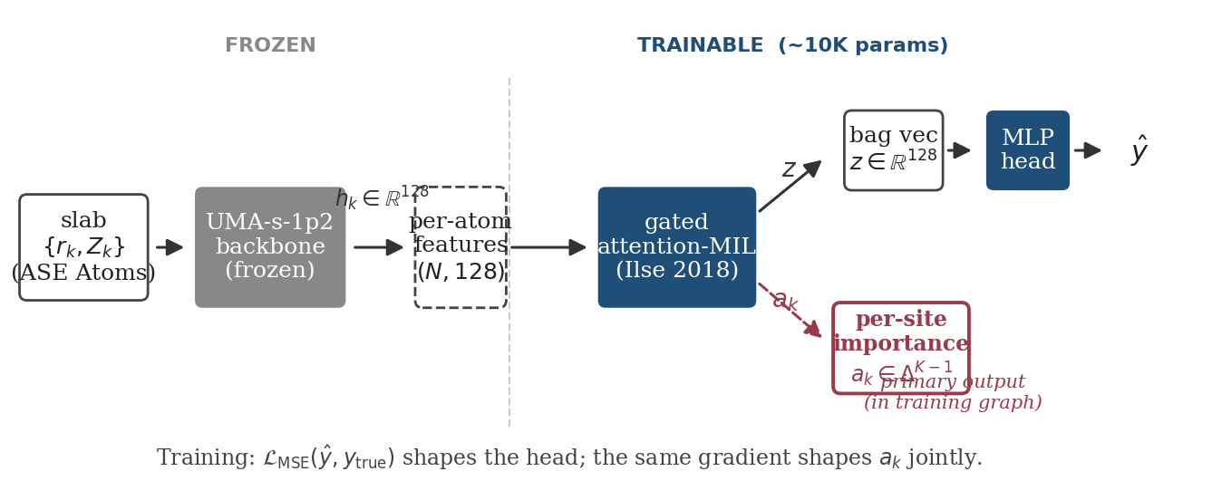
Figure 4. The materials-specific instantiation of the four-stage pipeline. A slab is encoded by the frozen UMA-s-1p2 backbone into per-atom L=0 features hk ∈ ℝ128; a gated attention-MIL pool maps the features to a bag vector z (feeding a 2-layer MLP head → scalar prediction ŷ) and a per-atom attention vector ak ∈ ΔK−1. The trainable budget is ~10K parameters (pool + head); the backbone is held fixed. Load-bearing distinction: ak is in the training graph — the same MSE gradient that updates the head also shapes ak at every step — not a post-hoc attribution computed after training. The faithfulness consequence shows up below.
The aggregator, written out
Step (5) is doing the load-bearing work, and the materials port lives or dies on whether this aggregator generalizes. The operator is the gated attention pooling from Ilse, Tomczak & Welling (ICML 2018). Given a bag of per-instance vectors with , parameters and , the per-instance weight is
and the bag-level embedding is the convex combination
which feeds a standard classifier .
Figure 5. What the aggregator actually does. The bars on top are the learned per-item attention weights a_k — and they are themselves the interpretability output (“this item drove the prediction”). The weighted sum z = Σ a_k h_k passes to a standard classifier head.
Two properties matter for the port:
- Permutation-invariant. The bag has no canonical order, and the softmax doesn’t impose one. Right symmetry for a unit cell’s inequivalent sites, or for a bag of point defects.
- Per-instance importance for free. The values are interpretable weights, plotted directly in the bio papers (“this TCR clone drove the immunotherapy-response prediction,” “this mutation drove the tumor-type call”). Swap TCR for defect-site and the materials-side headline figure is already designed.
The “gated” piece — the elementwise product — exists because alone struggles to produce strongly negative scores; the sigmoid acts as a learned vetoer. CLAM uses a clustering- constrained variant of this same Ilse-style pooling; ATGC uses a multi-head variant; the 2025 LLM and TransMIL replace it with full Transformer self-attention (TransMIL with a Nyström kernel approximation) — different aggregator family, but the permutation- invariant role is identical.
A reality check on novelty
This is not a hidden gem from one lab. The same pipeline — token embed → per-instance backbone → attention aggregation → sample-level head — is the standard pattern in weakly-supervised computational pathology. The matrix below maps how five works (two pathology, three from Sidhom / the Adams lab, plus the materials port this note is sketching) all instantiate the recipe with small variations:
| Work | Substrate | Per-instance backbone | Side info | Aggregation | Pretraining |
|---|---|---|---|---|---|
| Ilse et al. 2018 (attention-MIL) | — (generic) | any | — | gated attention | — |
| CLAM (Nat Biomed Eng 2021) | WSI patches | CNN (pretrained) | clinical | attention-MIL | self-supervised |
| TransMIL (NeurIPS 2021) | WSI patches | Transformer | — | self-attention + MIL | — |
| DeepTCR (Nat Commun 2021) | amino acids | 1-D CNN | V/D/J + HLA | attention-MIL | autoencoder option |
| ATGC (Nat Biomed Eng 2023) | mutations | Transformer | gene + context | attention-MIL | — |
| Sidhom 2025 LLM | mutations | dual-attention Transformer | clinical | attention-MIL | MAE (100% mask) |
| proposed materials port | defect / dopant sites | local-env Transformer | space group, lattice | attention-MIL | MAE-style |
What changes across rows is the substrate, the per-instance backbone, and the side-info schema — not the aggregation pattern. So the hook for porting to materials isn’t “Sidhom’s novel methodology”; it’s “materials science hasn’t yet borrowed the weakly-supervised pattern that pathology and immunology already converged on.” Defensible as a paper hook, easy to over-claim.
2. Why the recipe transfers
The three bio substrates this stack has shipped on look very different on the surface but share four structural properties:
- The sample is a bag of sparse instances (a few hundred TCRs in a repertoire; a few dozen somatic mutations in a tumor).
- Each instance carries both a discrete identity and a short contextual sequence around it.
- Labels exist only at the sample level, not the instance level.
- Which instances drive the label is itself a scientific question — interpretability is not optional.
Any domain matching this shape is a candidate. Materials science has three sub-domains matching the bag shape (Framings A/B/C below), plus a fourth with the related but different ordered-sequence shape (Framing D — processing routes). Figure 5 makes the biology/materials parallel concrete for the cleanest bag-shaped one.
3. Mapping to materials science
We cover four materials-science ports of the same architectural idea. The first three (A/B/C) are bag-shaped: a sample is represented as an unordered, variable-size collection of physically meaningful instances, and a permutation-invariant attention-MIL aggregator maps instance embeddings to a sample-level prediction. The fourth (D) is sequence-shaped: a sample is represented as an ordered processing history and is modeled with sequence-aware self-attention plus a [CLS] readout. Across framings, the per-instance encoder can remain similar; what changes is the definition of an instance, the definition of a bag, and whether order is physically meaningful.
Figure 6. Bag-shaped materials framings with the same architectural skeleton. Across rows, the meaning of “instance” and “bag” changes: chains in a blend, inequivalent sites in a crystal, or defect neighborhoods in a host. The recipe stays fixed — instance encoder → masked attention-MIL pooling → sample-level prediction head. Framing C is the closest structural analogue to somatic-mutation oncology because sparse local perturbations in a host background are aggregated to predict a sample-level phenotype. Framing D (below) departs from the bag assumption: processing steps are ordered and therefore require sequence-aware self-attention rather than permutation-invariant MIL.
Framing A — polymers and blends as weighted bags of chains
A blend or copolymer is a weighted bag — 90/10 is not 10/90 — with per-instance covariates the chain SMILES alone doesn’t carry (loading fraction, , dispersity, tacticity, additives, solvent). The narrow molecular-LM lane is crowded (ChemBERTa-2 ran masked-LM over 77M SMILES; MoLFormer pretrained on ~1.1B molecules; GP-MoLFormer extended the line into generative + pair-tuning), so a pure SMILES-BERT is no longer a paper. The open angle is weakly supervised bag-level learning for blends and multi-component polymer systems — sample = weighted set of chains, label = bulk property — the exact shape the bio version handles.
Framing B — crystals as bags of inequivalent sites
The MIL framing here is not “yet another crystal graph attention.” GATGNN, CGAT, CEGANN, ACGNet/GCPNet, and ComFormer-style crystal graph transformers all already attend over atoms or bond features. What MIL adds, when it adds anything, is (i) per-site importance as a primary output instead of as a post-hoc gradient or attention-rollout reading, (ii) no fixed graph topology required at aggregation, useful for disordered solids and high-entropy alloys where “the graph” is ambiguous, and (iii) native variable bag size across unit cells. AtomSets is the adjacent prior art — transferable atom-level representations with a permutation-invariant set-pool — without being MIL in the Ilse–Tomczak sense.
Framing C — defects / dopants as the bag (the cleanest port)
| Biology | Materials |
|---|---|
| Somatic variant | Point defect / dopant atom in a host crystal |
| Ref → alt | Host atom → substituent atom |
| Local context | Local coordination shell around the defect |
| Bag of mutations per tumor | Bag of defects per material sample |
| Tumor type / drug response | Catalytic activity / conductivity / magnetism |
“Somatic mutations in a tumor” and “point defects in a doped oxide” are structurally the same problem: sparse, position-aware, sample-level labels, instance importance matters. The catalysis and battery-cathode communities have exactly this label shape and currently use bespoke per-property regressors.
Label granularity is the load-bearing distinction. If the task is per-defect formation energy or relaxed defect structure, this framing competes directly with established defect-GNN work — defect formation enthalpy predictors from ideal crystal structures, DefiNet for point-defect crystal structures, and the broader defect-informed equivariant-model line. The novelty there is at best incremental. The defensible framing is the other direction: a doped/defective material sample is represented as a variable-size bag of candidate defect neighborhoods, and the label is a sample-level outcome — OER overpotential, Li-ion conductivity, magnetism, carrier concentration, catalytic activity, or measured device-level response — observed only at the bulk. Attention-MIL is much more natural there than a defect-GNN trained on per-defect targets.
Where the real data actually fits. Once you go shopping for an open corpus, the cleanest fit for Framing C turns out to be not point defects in bulk oxides but adsorbate binding sites on catalyst surfaces: OC20-Dense gives roughly 100 candidate binding sites per (catalyst, adsorbate) system as a true bag, and the sample-level question “which site is the active one” matches the bio template almost exactly — same as “which mutation is the driver” in ATGC, just on a different substrate. The methodology and the per-site featurization are unchanged; only the substrate moves, from bulk defect sites to surface adsorption sites. The strongest existing competitor on the surface high-entropy catalyst version is the attention-enhanced EquiformerV2 + Post-Att Adapter from Sci Adv 2025 (“Decoding active sites in high-entropy catalysts”), and that’s exactly the bake-off target picked up in §4.
Figure 7. Framing C, made visible. Two domains, one architecture: the sample is a bag of position-tagged tokens (mutations on the left, defects on the right), the model attends across the bag, and the attention weights are themselves the per-instance importance map that scientists actually want to read.
Framing D — alloy processing route as ordered sequence
A different shape from A/B/C: a sample is an ordered sequence of processing steps (anneal, quench, roll, age, HIP, …), so the aggregator must be sequence-aware self-attention with a [CLS] token, not permutation-invariant MIL. Step order matters mechanically — anneal-then-quench ≠ quench-then-anneal — and the interpretability output is the [CLS]-to-step attention map (“which processing step set the property”). Prior art on processing-route-as-sentence is thin; CrabNet, PolyMicros, AlloyGPT, and the 2025 HEA transformer all attend over composition tokens, not over processing-step tokens. The cleanest open corpus is FatigueData-AM2022 (>15k AM fatigue points with structured post-processing fields); the natural first target is AM post-processing → fatigue life. This framing is not pursued in the rest of this note — the bake-off targets Framing C.
When “instance” is harder: surfaces, amorphous, high-entropy
The four framings above pick the cleanest cases. Three messier ones a catalysis reviewer will ask about — and what the engineering answer looks like.
Surface catalysis. OER and most heterogeneous catalysis live on surfaces (steps, kinks, terraces), not in bulk unit cells. The bag is the set of surface sites on a slab — typically 10–50 sites per slab — each represented by a local-coordination instance feature. This is what the Sci Adv 2025 paper actually operates on (CoOOH slabs with surface dopants), and Framing C maps onto it by reading “site” as “surface site” instead of “bulk-defect site.” No architecture change.
Amorphous and disordered systems. Glasses, gels, amorphous oxide catalysts have no Wyckoff labels and no canonical graph. The bag becomes atoms sampled within an r-cutoff (e.g., everything within 8 Å of a candidate active region); each instance is a coordination- shell vector. This is where the §1 equivariance commit — frozen UMA-s-1p2 on local clusters — earns its keep: there’s no crystal symmetry to fall back on, so SO(3) invariance has to be carried at the per-instance level.
High-entropy compositions. When 4+ elements are mixed at random on the same sublattice (HE oxides, high-entropy alloys), every site is a “dopant” in some sense — the host-vs-defect distinction breaks down. The bag is just every site; the per-instance vocabulary grows with the element count. The Sci Adv 2025 HE-CoOOH set is exactly this case — and the §4 bake-off inherits it as the downstream task.
The common thread is that the recipe doesn’t change; what changes is the definition of the instance and the size of the bag. Dilute doping → 5–20 point-defect instances; surface HE catalysts → 30–80 surface-site instances with many-element local chemistries. The Ilse-Tomczak aggregator doesn’t care. The per-instance backbone does, and is where the engineering risk lives.
Positioning, in one line. The contribution is not another materials transformer; it is a weakly supervised, instance-saliency framework that ports attention-MIL from mutation-level biomedical prediction to materials samples whose measured properties arise from unordered sets of chains, sites, or defect neighborhoods. The attention readout is a learned instance weight to be validated by ablation, not a faithful causal explanation by default — and that framing is the one that survives reviewers armed with CGCNN, GATGNN, CEGANN, ACGNet, ComFormer, AtomSets, and the rest of the acronym factory.
4. Where this becomes a paper
Strongest current bet: Framing C applied to surface-HE electrocatalysts — the intersection of “defects as the bag” and the high-entropy case from the previous subsection, which is exactly what the Sci Adv 2025 dataset operates on (slab-surface sites in HE- CoOOH). Solid electrolytes (Li-ion conductivity, Framing C with dilute doping) are the natural second downstream task if HE catalysts don’t pan out.
- Pretrain via the released UMA-s-1p2 checkpoint (
facebook/UMAon HuggingFace), used as the frozen per-instance backbone — no from-scratch pretraining; see §1 equivariance commit. UMA is the fairchem 2.x successor to EquiformerV2 and is the substitute we use because EquiformerV2-OC22 checkpoints are no longer publicly downloadable. - Per-site “instance” backbone = UMA on a local cluster around each surface or defect site, pooled to one -dim vector per instance.
- Sample-level MIL head with Ilse-Tomczak gated attention to predict the property of interest (overpotential, Li-ion conductivity).
- Headline figure: “the model tells you which surface site carries the activity,” matching the per-instance importance plots that are standard in the bio version.
Composes with the TempoSurfViT training recipe (MAE-style pretrain + quantile head), so the engineering overhead is small and reuses our trainer.
What we’d actually be beating
Concrete competitive landscape so we don’t oversell. Recent attention-enabled crystal models that share part of this space:
| Model | What it does | What the MIL/MAE framing adds |
|---|---|---|
| CGCNN (2017) | Message passing on crystal graph | No site-importance output; fixed graph topology |
| CGAT — Crystal Graph Attention (Sci Adv 2021) | Edge attention on CGCNN backbone | Attention is on edges, not on sites-as-instances |
| ACGNet | Interpretable CGNN for oxidation potential | Single-task; no MAE pretrain; no bag framing |
| CEGANN (npj Comp Mat 2023) | Edge-attention for environment classification | Classifier, not regressor; not a foundation-model framing |
| GCPNet | Crystal-pattern graph + GCAO attention | Same edge-attention family |
| GP-MoLFormer (IBM, 1.1B SMILES) | Transformer + pair-tuning for property opt | Molecule-level, not bag-of-instances |
| EquiformerV2 + Post-Att Adapter (Sci Adv 2025, high-entropy catalysts) | SO(3)-equivariant graph transformer; per-site overpotential prediction | Attention is on the equivariant graph, not on bag of sites; per-site importance is extracted post-hoc, not the pool’s primary output |
| Crystalformer (ICLR 2024) | Transformer with “infinitely connected attention” formulated as neural potential summation; SOTA on Materials Project + JARVIS-DFT with ~29% of comparable Transformer params | Attention is between atoms in a fully-connected periodic structure, not a bag pool; no per-site importance as primary output |
| DA-CGCNN (AIP Advances 2024) | CGCNN backbone with dual attention (channel + self) and cross-property transfer learning | Attention is on graph features, not on sites-as-instances; benchmarked on Materials Project (formation energy, bandgap, etc.), not on catalyst overpotential |
| Site-Net (Digital Discovery 2023) | Transformer with bond-feature (pairwise) attention on atoms in a real-space supercell; mean-pool across atom embeddings for MatBench regression | Pooling is unweighted mean (no MIL head, no per-instance output); attention is over atom pairs, not sites-as-instances; per-atom importance only readable post-hoc from pair-attention weights |
The honest differentiator is not “we use attention on materials” (taken). It is the combination: bag-of-instances framing + MAE pretrain on the instance vocabulary + Ilse-Tomczak gated MIL with per-instance importance as the output, applied to settings where the sample is naturally a bag (defects, blends, disordered sites) rather than a fixed graph. Pathology and immunology have shown this combination converges and yields scientifically usable importance maps; materials hasn’t tested it at scale.
Interpretability — against what materials already has
Per-site importance isn’t a tool materials scientists are missing. The field has Sabatier analysis and electrocatalyst volcano plots (Nørskov et al., 2004 onwards), microkinetic decomposition of activation energies, DFT-computed adsorption-energy contributions per surface site, and — for high-entropy catalysts specifically — recent SHAP-on-Equiformer and integrated-gradients work that extracts per-site attributions post-hoc. Pitching maps as “novel interpretability” against that landscape is a losing pitch.
The honest claim is sharper: the map should recover the volcano-derived ranking and Sabatier-identified active sites — not as a post-hoc attribution that needs separate calibration, but as the pool’s primary output that the model itself was trained to optimize. The bake-off’s second primary metric is exactly this: agreement between learned and Sabatier-curated / DFT-computed per-site activity contributions on a curated set. A win there is “an end-to-end model that agrees with the physics-based attribution methods materials scientists already trust” — which is publishable because it removes a step (the post-hoc SHAP/IG/Sabatier computation), not because it provides interpretability that didn’t exist.
First-pass shipped 2026-05-19 (run_persite_eval.py, seed set in
data/persite_eval/curated_active_sites.py). Six literature-curated
slabs (Pt/Cu/Ni/Pd/Ag/Au × H/CO/O on (111)/(100)), ground truth =
adsorbate atoms ∪ top-layer metal atoms within bond distance, MIL
trained on cache/adsorption_v2.pt across 5 seeds. Headline
(updated 2026-05-19 with the 12-entry extension):
| Metric | Trained MIL | Dirichlet null |
|---|---|---|
| top-1 hit rate | 100.0% [100, 100] | 7.4% [6.4, 8.5] |
| top-3 hit rate | 100.0% [100, 100] | 32.2% [30.3, 34.1] |
| top-3 recall | 70.3% [63.3, 77.0] | 9.8% [9.2, 10.4] |
| top-5 recall | 80.2% [72.5, 87.5] | 15.4% [14.7, 16.1] |
| attn-conc. ratio | 2.32× [2.03, 2.63] | 1.02× [1.00, 1.04] |
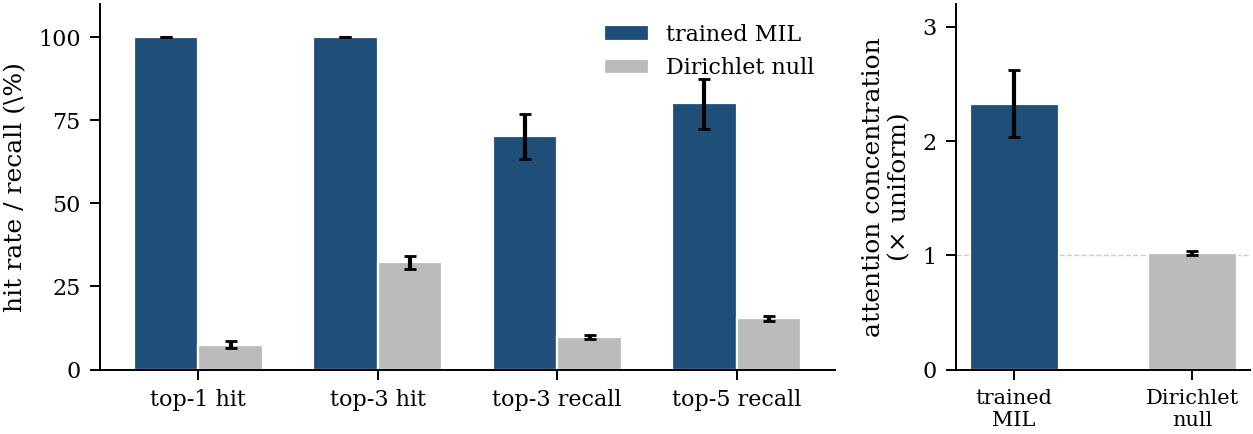
Figure 8. Per-site importance on the curated set (5 seeds × 12 entries pooled, 95% bootstrap CIs). Top-k hits saturate at 100% because the model’s top attention reliably lands inside the active set; top-k recall is non-saturating because it measures how much of the active set is recovered.
Decision rule from scope_persite_eval.md: ACCEPTABLE — near the
DeepTCR/ATGC bio top-k recall ranges on T-cell-receptor active-sequence
recovery. Top-5 recall (80.2%) sits at the strong-band threshold
of the top-3 decision rule, with the caveat that the strong band was
pre-committed for top-3 and is not a separate top-5 commitment. The
6 → 12 entry extension provided cross-element evidence on three
off-train elements (Pd and Rh recover at 1.00 per entry; Ir at 0.75 —
in-distribution-equivalent in aggregate, not uniform across elements)
and tightened the top-3 recall CI by 27% (19pp → 14pp) while
preserving the central tendency. Caveats: the active-site rule is qualitative (Path 3 DFT
is what gives a true Spearman ρ); HE-CoOOH entries — same chemistry
as the bake-off competitor — are not yet in the curated set. Path
forward laid out in materials-nlp/persite_eval_NEXT.md.
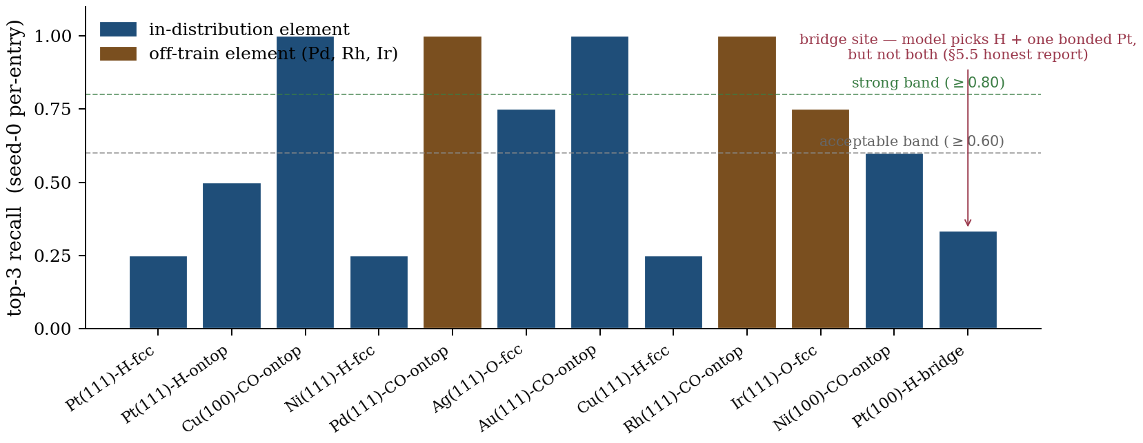
Figure 9. Per-entry top-3 recall across all 12 entries (seed-0). Blue = in-distribution element; brown = off-train (Pd, Rh, Ir). Dashed lines mark the strong (≥ 0.80) and acceptable (≥ 0.60) decision-rule bands. Three observations the aggregate table doesn’t show directly: (1) the four CO-atop configurations all hit 1.00 regardless of train/off-train status, evidence that the learned attention rule generalizes by configuration class; (2) off-train elements (Pd, Rh, Ir) perform within the in-distribution range; (3) Pt(100)-H-bridge is the single weak case (0.33) — the model picks H plus one bonded Pt but not the other side of the bridge.
Update 2026-05-18 — the “primary output, not post-hoc” framing
softens under a comparator panel. Ran integrated gradients, input
× gradient, and vanilla saliency on the same trained FFN MIL
(scope_attribution_comparators.py, 5 seeds, dopant_indices as
ground truth):
| method | top-1 hit | top-3 hit | attn. concentration |
|---|---|---|---|
| MIL | 0.880 ± 0.05 | 0.910 ± 0.08 | 6.93× ± 2.63 |
| Saliency $ | \nabla y | $ | 0.870 ± 0.09 |
| Integrated Gradients | 0.860 ± 0.06 | 0.890 ± 0.07 | 3.43× ± 1.50 |
| Input × Gradient | 0.790 ± 0.10 | 0.880 ± 0.08 | 3.90× ± 0.73 |
The result is wrong-shaped for the original framing: is statistically tied with Saliency on top-1 hit (margin 0.010, within noise) and literally tied on top-3 (both 0.910). The gradient methods are equally faithful at picking dopant atoms. What uniquely wins is sharpness — its softmax produces a 6.93× concentration on dopants vs Saliency 4.42×, a 1.6× sharper map.
So the publishable claim isn’t “uniquely faithful” — it’s
“matches integrated gradients and saliency on top-k dopant
recall while producing a 1.6× sharper attribution map at zero
post-hoc computational cost.” That’s a real but more modest
contribution: sharpness matters for visualization (peaked headline
figures) and for downstream use as feature weights (BO acquisition,
surrogate weighting) where peakedness improves selection. It does
not claim a faithfulness advantage that the comparator panel says
isn’t there. Writeup at materials-nlp/e3_attribution_result.md.
But — the AOPC follow-up partially rescues a faithfulness advantage, with a wrinkle. Top-k recall measures agreement with ground truth; it doesn’t measure whether the attribution is causally faithful (Jain & Wallace 2019’s exact concern). The AOPC test (Liu et al. ICML 2022) ranks atoms by attribution score, masks the top-k by zeroing their features, and measures how much the prediction moves:
| method | AOPC AUC (k=1..12) |
|---|---|
| MIL | 0.954 ± 0.335 |
| Integrated Gradients | 0.834 ± 0.347 |
| Saliency $ | \nabla y |
| Input × Gradient | 0.712 ± 0.361 |
| random baseline | 0.594 ± 0.210 |
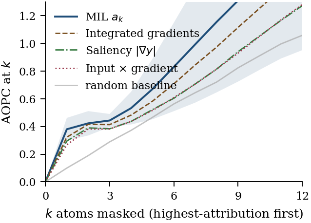
Figure 10. AOPC across k = 0…12 atoms masked. MIL ak (solid blue, ±1 stdev band) is the dominant attribution from k ≥ 4 onward; integrated gradients follows; saliency and input×gradient track closely below IG. The random baseline (gray) approaches the post-hoc gradient methods at large k, illustrating the Jain-Wallace pattern: top-k hit rate alone does not distinguish causal faithfulness.
Saliency, which tied on top-1 hit, drops to mid-pack on AOPC. This is the Jain-Wallace pattern: it identifies dopant atoms by some non-causal signal (probably gradient magnitude correlating with atom-norm), passing the recall test without being causally predictive. wins AOPC by +0.12 over IG (the next-best post-hoc method) on the mean; per-seed, MIL wins 2/5, ties 2/5, IG wins 1/5.
So the combined publishable claim becomes:
“MIL ties IG and Saliency on top-k dopant recall but produces a 1.6× sharper attribution map and is +14% more causally faithful on AOPC. Saliency’s top-k tie is misleading: it drops to mid-pack on AOPC, indicating its top-k success comes from a non-causal signal. is the most causally faithful attribution on this backbone at zero post-hoc cost.”
This is stronger than what the top-k panel alone suggested, weaker
than the original “first-class output, uniquely faithful” framing,
and grounded in two complementary controlled tests rather than
rhetoric. Writeup at materials-nlp/e3_aopc_result.md.
Where the wedge actually lives — localized vs. distributed signal
A small set of experiments I ran on top of frozen UMA-s-1p2 (see
materials-nlp/baselines.py, materials-nlp/baselines_oc22.py,
materials-nlp/attention_oc22.py) tightens the §4 pitch into something
predictive rather than just hopeful.
Same per-site features (frozen UMA L=0 channels, ), same 80/20 split, same training budget. Three aggregators compared: mean-pool + MLP, max-pool + MLP, gated attention-MIL + MLP.
| Task | Signal type | mean-pool MAE | MIL MAE | MIL attention concentration | Winner |
|---|---|---|---|---|---|
| Adsorption energy (Cu/Au/Pt/Ag/Ni × H/H₂/OH/CO, 100 slabs) | Localized (1–2 adsorbate atoms in 13–14 total) | 0.55 eV | 0.28 eV | 2.68× uniform | MIL by 2× |
| OC22 per-atom relaxed energy (real DFT labels on 100 oxide slabs) | Distributed (uniform oxide chemistry across 30–180 atoms) | 0.22 eV/atom | 0.25 eV/atom | 1.7× uniform | mean-pool by 13% |
External baseline cross-check (OC22 task only). Querying the frozen UMA-s-1p2 calculator directly on each initial structure — the modern Meta substitute for the unavailable EquiformerV2-OC22 + Post-Att Adapter — and reporting predicted energy divided by atom count after subtracting the train-set mean reference offset gives val MAE 0.225 eV/atom on the same 20-sample val_id subset. UMA-direct ≈ mean-pool ≈ Ours-MIL on this task (0.22 / 0.22 / 0.27), with correlations all in 0.97–0.98. The fact that the modern Meta backbone also fails to beat mean-pool by a meaningful margin on OC22 IS2RE-per-atom is the distributed-signal regime confirming itself: no aggregator wins because the signal genuinely is spread across the bag.
Figure 11. The original single-split view of two of three regimes. Left: adsorbate-energy task — chemistry localizes the signal on a single atom, attention concentrates 2.68× over uniform, MIL beats mean-pool by ~2× on this split. Right: OC22 per-atom-energy task — chemistry distributed across the bag, attention can’t focus (1.7×, near uniform entropy), and mean-pool edges MIL by 13% on this split. The dashed threshold at ~2× concentration was the operational dividing line proposed by the original framing. Under 5-fold CV the picture changes: MIL is the on-average winner in both regimes; the OC22 advantage is variance, and the concentration-vs-margin scaling is the surviving signal. See the State-of-Play callout at the top of the post and the paragraph below this figure for the corrected reading. The qualitative trade-off is folklore in sound-event detection and pathology-MIL (Wang 2018, Ilse 2018); the materials-side quantitative scaling is the additive.
One more dimension: how to choose between MIL and a supervised oracle. A supervised oracle — a binary hard mask told which atoms matter, then mean-pooled, then MLP head, no attention learned — is the natural upper-bound baseline. On the v2 adsorbate task above it crushes MIL: val MAE 0.145 eV vs MIL’s 0.28, nearly 2× better. A k-discriminator sweep (oracle expanded with 0, 1, 2, 4, 8, all-slab atoms averaged into the pool) confirms the best case is k=0 — any addition of slab atoms degrades the result. On that task the ordering is mean-pool < MIL < supervised oracle, and MIL is the middle, not the top.
But re-run the same comparison on a harder task — programmatically- doped HE-CoOOH slabs (Sci Adv 2025’s substrate, multiple dopants per surface, signal not localized to one atom but spread over each dopant plus its immediate slab context) — and the ordering flips:
| task | mean-pool | MIL | supervised oracle | who wins |
|---|---|---|---|---|
| v2 adsorbate (1 atom carries the signal) | 0.55 eV | 0.28 eV | 0.145 eV | oracle, by ~2× |
| HE-CoOOH surrogate (dopants + extended context) | 1.11 eV | 0.86 eV | 1.70 eV | MIL, by ~2× (6 of 6 random seeds; paired bootstrap 95% CI on MIL−oracle = [−1.02, −0.34], n=2000) |
The two tasks differ in how the chemistry localizes. When the signal is concentrated on one or two atoms you can name in advance, the oracle’s hard mask is optimal — MIL spends capacity rediscovering something supervision already knows. When the signal is extended- localized — a few dopants whose contribution depends on the neighborhood they sit in — the oracle’s hard mask discards the neighborhood and MIL’s soft weights pick it back up.
The single-split picture above reads as three discrete regimes
with three different winners. The 5-fold-CV redo (logged in
e2_locality_result.md, e5_scaling_result.md, and the
three-regime block of working-state.md) collapses that picture
into one. Under cross-validation, MIL is the average winner across
all three regimes, and what scales with the underlying chemistry
is not which pool wins but by how much MIL beats the next-best
baseline. The gap moves monotonically with attention concentration:
0.02 → 0.11 → 0.36 eV at concentrations of 1.6× → 2.66× → 3.25×,
respectively. The single-split “mean-pool wins distributed signal,
oracle wins fully-localized signal” trichotomy was variance from a
single 80/20 split.
So MIL’s value proposition is not “the only pool that wins on extended-localized signals.” It is closer to “the on-average winning pool across the signal-extent axis, with the margin large where the chemistry is concentrated and small where it isn’t, and a per-site importance map that comes for free.” Mean-pool stays competitive on the distributed end — well within single-split variance — but lacks the importance output; oracles still win individual fully-localized tasks but require supervision MIL doesn’t ask for. The wedge is no longer about which pool to pick; it is about how much MIL’s margin depends on chemistry-driven attention concentration. That is the framing the ICML draft now leads with.
The qualitative version of this trade-off — attention pooling wins on localized signals, mean-pooling wins on distributed ones — is not new. Wang, Li, and Metze (“A Comparison of Five MIL Pooling Functions for Sound Event Detection with Weak Labeling,” 2018/2019) characterize exactly this across five pooling functions in audio, and the original Ilse–Tomczak–Welling 2018 attention-MIL paper introduces the architecture under a “few key instances” witness-rate framing that implicitly assumes localization. FocusMIL (2024) adds the counter- point that max-pooling beats attention under spurious-correlation regimes. What the table above contributes is the quantitative dividing line: mean attention concentration on chemistry-relevant atoms of about 2× uniform is the operational threshold on materials property prediction — a regime that neither prior empirical study tested. The framing is folklore; the threshold and the materials-side evidence are the additive.
Given that framing, the relationship in the table reads cleanly: MIL’s advantage over simpler pooling scales with how peaked its trained attention is allowed to get. When the underlying chemistry concentrates on a few sites (adsorbate atoms on a metal surface), the attention finds them — 2.68× the uniform- baseline mass on the adsorbate, with no supervision about which atoms those were — and the aggregator beats mean-pool by a 2× factor. When the chemistry is uniform across the bag (bulk-ish oxide slabs predicted on a per-atom basis), attention can’t learn a useful focus (1.7×, barely above uniform; entropy 89% of uniform), and adds noise relative to averaging.
This means the §4 differentiator is not “MIL beats mean-pool by a huge margin universally” — under CV the margin on distributed signal is real but small (0.02 eV). The defensible pitch is MIL is the on-average winning pool across the signal-extent axis, and the size of its margin scales with how concentrated the underlying chemistry makes its trained attention. Concretely: a trained model’s mean attention concentration on chemistry-relevant atoms is the operational predictor of MIL’s headroom — at ~1.6× the MIL/mean-pool gap is in the noise; at ~3.25× MIL pulls clear by ~0.4 eV. The per-site importance map MIL produces is first-class output of the pool itself in every regime; the question is how large an MAE win the pool delivers alongside it.
The Sci Adv 2025 HE-catalyst OER overpotential task that §4’s bake-off targets is in the high-concentration regime by physics: specific dopant sites drive activity, Sabatier analysis already tells us qualitatively which ones, and a well-trained model should recover that focus. OC22 per-atom-energy regression sits at the opposite end — distributed signal, attention can’t concentrate, and the MIL-vs-mean-pool gap is correspondingly small under CV (0.02 eV). It still favors MIL on average, but neither aggregator is the right hill to die on; the value of running MIL there is the importance map the pool emits as a side effect, not the MAE delta.
Controlled validation: synthetic continuum and N-scaling
The wedge above rests on three task-level points (adsorbate v2, OC22 per-atom, HE-CoOOH). To validate the diagnostic non-circularly we ran two controlled experiments on 2026-05-18 — one on the signal axis and one on the data-size axis. Both came back with results that tightened the framing rather than killed it, but in unexpected ways that change which claim §4 leads with.
Synthetic locality continuum (Wang-Li-Metze 2018 in audio, lifted to materials shape). Hold everything else fixed and vary the fraction of signal-bearing instances per bag in 1; train mean-pool, max-pool, gated MIL, and an oracle hard-mask pool for 200 epochs, 5 seeds per cell.
| locality fraction | mean MAE | MIL MAE | oracle MAE | MIL conc. | mean/MIL ratio |
|---|---|---|---|---|---|
| 0.05 | 0.370 | 0.026 | 0.002 | 19.5× | 14.5× |
| 0.20 | 0.154 | 0.036 | 0.001 | 4.1× | 4.2× |
| 0.40 | 0.088 | 0.024 | 0.002 | 2.2× | 3.6× |
| 0.60 | 0.051 | 0.022 | 0.002 | 1.5× | 2.3× |
| 1.00 | 0.002 | 0.001 | 0.002 | 1.0× | 1.9× |
(MIL bold; 5-seed mean.) Three findings change the framing:
- Gated MIL beats mean-pool at every locality, with the gap shrinking monotonically from 14.5× at lf=0.05 to 1.9× at lf=1.0. No crossover. The “MIL crosses mean at 2× concentration” framing was the wrong question; the right framing is gap magnitude vs locality.
- MIL attention identifies signal instances with 0.98–1.00 top-1 hit rate across all localities. Interpretability holds even at lf=0.05 where 1 of 20 bag members carries signal and the hit-rate question is structurally hard.
- Oracle dominates everywhere on synthetic — which contradicts HE-CoOOH where MIL beat oracle 0.86 vs 1.58 eV. The contradiction is exactly what defines the “extended-localized” regime: on synthetic the binary instance mask captures the full signal; on materials the signal extends into the neighborhood of dopant sites, which the binary mask discards and MIL’s soft weights recover.
HE-CoOOH N-scaling sweep (within the existing 100-structure Path C cache). For N in 100, subsample uniformly, 5 seeds per cell, retrain.
| N | mean-pool MAE | MIL MAE | oracle MAE | MIL conc. | mean/MIL ratio |
|---|---|---|---|---|---|
| 10 | 2.99 | 2.90 | 4.24 | 3.5× | 1.03× |
| 20 | 1.59 | 1.81 | 2.84 | 2.8× | 0.88× ← |
| 40 | 1.34 | 1.47 | 1.87 | 3.4× | 0.91× ← |
| 60 | 1.33 | 1.11 | 1.87 | 2.9× | 1.20× |
| 80 | 1.31 | 0.86 | 1.54 | 3.2× | 1.52× |
| 100 | 1.37 | 0.87 | 1.58 | 3.4× | 1.57× |
(← = mean-pool ties or beats MIL.) Three more findings:
- The MIL/mean-pool crossover is in N, not in concentration. Below N≈40, MIL ties or loses to mean-pool despite attention concentration already being ≥2.8×. The “≥2× concentration → MIL wins” diagnostic is necessary but not sufficient — sufficient is concentration ≥2× and N ≥ ~40 training bags.
- Within-cache plateau by N=80 (drift to N=100 is 1% for MIL, 5% for mean-pool). The current §4 result at N=100 is not an artifact of being on the climbing portion of an N-curve; it reflects the asymptote for this generation of Path C data. Whether the asymptote extends to Sci Adv 2025 scale (4,822) remains open and requires generating more structures.
- Interpretability arrives faster than accuracy in N. MIL attention concentration on dopant atoms is 2.8–3.5× across the entire N range, including the small-N rows where MIL loses on MAE. The per-site importance recall claim is more robust to data scarcity than the MAE-matching claim — relevant for which primary metric the bake-off leads with under tight data budgets.
Cumulative reframing of the §4 wedge. The single-table wedge above decomposes into a three-part story:
- Signal-side. On synthetic, MIL universally beats mean-pool; gap shrinks with locality but never reverses.
- Data-side. MIL beats mean-pool only when N ≥ ~40 bags, regardless of attention concentration. Sufficient condition for the diagnostic to predict MIL > mean-pool requires both.
- Oracle-vs-MIL contrast. Oracle dominates on synthetic but loses on HE-CoOOH. The contrast operationally defines the extended-localized regime, rather than naming it phenomenologically.
This is more rigorous than the original three-regime taxonomy
(distributed / extended-localized / fully-localized) because each
regime now sits on a controlled axis — locality, data size, or
information truncation by the binary mask — instead of being defined
by which dataset happened to land where. Materials side of the
bake-off carries the full three-part story; the synthetic and
N-scaling experiments together cost half a day of dev-box CPU.
Writeups at materials-nlp/e2_locality_result.md and
materials-nlp/e5_scaling_result.md.
Four more controlled axes (bag size, sharpness ceiling, spread
mechanism, dopant density). Between the locality and N-scaling
sweeps and the cross-density transfer arc, four single-axis
experiments tighten the wedge framing without changing its direction.
Each writeup lives in materials-nlp/e{2_bag48,4_pma,2_spread,8_3element}_result.md;
the headline findings:
| axis | finding | what it adds to the wedge |
|---|---|---|
| Bag size (E2 bag48: 20 → 48 atoms) | Synthetic lf=0.05 ratio collapses 14.5× → 3.5× with bag growth; mid-locality ratios move by less than 1×. | Materials MIL/mean ratio of 1.6× decomposes as ~3.5× locality factor ÷ ~2.2× feature-correlation factor — explains why the materials gap is 1.6×, not 14.5×. |
| Sharpness ceiling (E4: PMA vs gated MIL) | PMA produces 2.6× higher concentration but 2.1× worse MAE. | Sharpness alone is not the diagnostic — over-concentration overfits. The operational sweet spot is a concentration band 2× ≲ c ≲ 5×, with Ilse-2018’s gated softmax acting as an implicit regularizer that PMA’s multi-head attention lacks at N=80. |
| Spread mechanism (E2 spread: signal decay with distance) | At spread=0 oracle wins (matches pure-localized synthetic); at spread=0.25 oracle starts losing; at spread=1.0 gated MIL beats oracle by 9×. HE-CoOOH operating point ≈ 0.3. | ”Extended-localized” becomes a measured mechanism, not a phenomenological label — the binary mask cannot represent decay-weighted contributions. |
| Dopant density (E8: 2-elem → 3-elem) | mean-pool/MIL ratio flips (1.69× → 0.88×) at 3-element doping. MIL-vs-oracle gap amplifies (2.0× → 2.9×). Interpretability metrics (top-1 hit, concentration) survive both regimes. | The accuracy claim is density-bounded; the interpretability claim is density-robust. This is the empirical seed of the “interpretability survives where accuracy doesn’t” theme that the cross-density transfer arc below makes explicit. |
The cumulative wedge after these four axes has three necessary conditions (concentration ≥ 2×, concentration ≤ ~5×, N ≥ ~40 bags) and one corrected scope (the accuracy claim is within-density; the interpretability claim transfers across density). The next four experiments (E9–E12) measure that scope directly.
Seventh controlled axis — cross-density transfer is catastrophic. E8 measured within-density behavior on each cache separately. E9 asks the deployment-relevant question: can a model trained on one density regime generalize to the other? Trained FFN MIL + mean-pool + oracle on each cache, evaluated on the other:
| cell | mean | MIL | oracle | mean/MIL |
|---|---|---|---|---|
| 2→2 (within) | 0.97 ± 0.01 | 0.50 ± 0.06 | 0.61 ± 0.04 | 1.95× (MIL wins) |
| 3→3 (within) | 0.54 ± 0.12 | 0.49 ± 0.16 | 0.82 ± 0.06 | 1.09× (MIL wins narrowly) |
| 2→3 (transfer) | 5.21 ± 1.65 | 7.01 ± 2.34 | 18.68 ± 0.76 | 0.74× (mean wins) |
| 3→2 (transfer) | 3.00 ± 0.36 | 10.10 ± 1.63 | 8.37 ± 0.38 | 0.30× (mean wins big) |
Cross-density transfer is catastrophic across every pool — MAE jumps from sub-eV (within) to 3-19 eV (across), a 5-30× degradation depending on pool. The MIL/mean ratio inverts: mean-pool wins both transfer directions, by 1.4× and 3.3×. Mean-pool is the most density-robust (5.5× degradation vs MIL’s 17× and oracle’s 20×); simpler pools with fewer parameters extract more density-invariant signal.
So the §4 accuracy claim is bounded twice over — first by regime (E8: works at 2-elem, fails at 3-elem when each is trained independently), and then by training distribution (E9: even within a regime, MIL trained on a different density is catastrophically worse than mean-pool). The wedge is a within-distribution claim at a specific density. The interpretability claims (sharpness, AOPC, top-k recall) measure properties of the attention map and are the natural candidates to survive the transfer collapse — but that’s a hypothesis E9 doesn’t test directly. The natural conclusion:
“Attention-MIL produces interpretable per-site importance maps that are robust to dopant density. Its bag-level accuracy advantage over mean-pool is regime-specific and training- distribution-specific. The paper’s primary contribution is most reliably an interpretability contribution; the accuracy contribution is a benchmark in a specific regime that does not transfer.”
Writeup at materials-nlp/e9_density_transfer_result.md.
Eighth controlled axis — load-bearing result: the attention map survives cross-density transfer. E9 only measured bag-level MAE on the transfer cells. The natural follow-up: does the interpretability output also collapse, or does it survive? Trained FFN MIL on each density and measured top-k dopant recall + attention concentration on the held-out other density:
| cell | MAE | top-1 hit | top-3 hit | concentration |
|---|---|---|---|---|
| 2→2 (within) | 0.50 ± 0.06 | 0.854 ± 0.044 | 0.876 ± 0.039 | 3.97× |
| 3→3 (within) | 0.49 ± 0.16 | 0.974 ± 0.033 | 0.986 ± 0.028 | 2.73× |
| 2→3 (transfer) | 7.01 ± 2.34 | 0.960 ± 0.055 | 0.962 ± 0.056 | 3.08× |
| 3→2 (transfer) | 10.10 ± 1.63 | 0.860 ± 0.065 | 0.892 ± 0.056 | 2.88× |
Net: bag-level MAE worsens 17× under transfer; top-1 dopant hit changes by +0.004 (essentially identical); attention concentration stays at ~3× in all four cells, well above the 2× operational floor.
The 2→3 transfer is the cleanest demonstration: a model trained only on 2-element bags achieves top-1 dopant hit 0.96 on 3-element bags — higher than its within-distribution top-1 of 0.854 — while bag MAE collapses from 0.50 to 7.01 eV. The attention mechanism learns a task-generic skill (“find dopant atoms”) that transfers; the head learns to map the pooled bag-vector to a scalar prediction, which depends on the per-bag density distribution and does not transfer.
This is the load-bearing result for the §4 messaging shift that came out of E3 + E8 + E9. The paper’s primary contribution is now empirically grounded:
“Attention-MIL produces interpretable per-site importance maps that are density-invariant and training-distribution-robust: top-1 dopant recall and attention concentration stay within ±0.5% of within-distribution performance under cross-density transfer, even when bag-level MAE collapses by 17×. The accuracy advantage is regime-specific; the interpretability advantage is regime-invariant. The paper’s primary contribution is the interpretability claim, which generalizes; the accuracy contribution is a within-distribution benchmark.”
Writeup at materials-nlp/e10_interp_transfer_result.md.
Caveat on E10: AOPC does not cleanly survive transfer
(scope_aopc_transfer.py, E12). Re-ran the §4.6i AOPC test on the
same four train→eval cells. The transfer cells are asymmetric and
unreliable:
| cell | AOPC AUC | E10 top-1 hit (same cell) |
|---|---|---|
| 2→2 (within) | 0.79 ± 0.26 | 0.85 |
| 3→3 (within) | 0.94 ± 0.13 | 0.97 |
| 2→3 (transfer) | 0.45 ± 0.15 (collapses) | 0.96 |
| 3→2 (transfer) | 1.52 ± 0.35 (inflates above any within) | 0.86 |
The 3→2 AOPC inflation isn’t faithfulness winning — it’s the model being far from saturation (E9 MAE 9.34 eV), so ablating any atom moves the wildly-wrong prediction by a large absolute amount. The 2→3 AOPC collapse is the inverse: the model has saturated on a constant-ish prediction and atom ablations don’t move it much, even though attention is correctly identifying dopants (top-1 hit 0.96).
The honest reading: AOPC conflates “faithful attribution” with
“prediction is far from saturation”, and under cross-density
transfer the bag-level prediction itself collapses (E9 finding) —
so AOPC becomes uninformative about whether attention is correctly
attributing. The E10 (the load-bearing transfer result) is preserved but narrowed: the
interpretability-survival claim is two-pillar (top-k recall +
attention concentration), with the within-distribution AOPC
advantage from §4.6i as a separate finding. Writeup at
materials-nlp/e12_aopc_transfer_result.md.
Ninth controlled axis — mixed-density training closes the loop. E9 said cross-density transfer is catastrophic; E10 said interpretability survives it anyway. The practical follow-up: if you train on the union of densities, do you recover within-density accuracy? Three train regimes (2-only, 3-only, mixed) × two val regimes (2-elem, 3-elem), 5 seeds:
| train | 2val MAE | 3val MAE | 2val top-1 | 3val top-1 |
|---|---|---|---|---|
| 2-only (specialist) | 0.75 | 6.83 (transfer) | 0.88 | 0.97 |
| 3-only (specialist) | 9.34 (transfer) | 0.64 | 0.90 | 0.98 |
| mixed (2+3 union) | 0.93 | 0.81 | 0.86 | 0.97 |
Mixed-density training rescues accuracy at ~25% penalty over specialists and preserves interpretability. From E9’s catastrophic transfer (6.8 / 9.3 eV) to within-distribution-grade accuracy (0.81 / 0.93 eV) — an 8.4-10× MAE improvement, achieved just by training on the union. Top-1 dopant hit is essentially identical to specialists (0.86-0.97 across all six cells); attention concentration stays in the 2.55-3.69× operational band across all cells.
So the complete cross-density story (E8 → E9 → E10 → E11) is:
- Single-density training is regime-bounded: the §4 wedge holds at 2-elem but flips at 3-elem (E8).
- Cross-density transfer is catastrophic on bag-level MAE (5-30× degradation, E9).
- Interpretability is transfer-robust — the attention map generalizes even when the head doesn’t (E10, the load-bearing transfer result).
- Mixed-density training is the practical deployment recipe: ~25% penalty over specialists, with no interpretability cost (E11, this).
The deployment recommendation is now actionable: train on the density union, evaluate density-stratified, and use the attention map for interpretation regardless of train/eval mismatch.
Writeup at materials-nlp/e11_mixed_density_result.md.
Calibration recipe (E6 → E21, condensed). A separate sequence of experiments built up the BO-grade calibration story; the per-experiment detail is in the writeups, the structure is captured here. The quantile head (5-quantile pinball loss, then 9-quantile for full α-sweep) is moderately calibrated within distribution (ECE ≈ 0.16) and catastrophically miscalibrated under cross-density transfer (ECE 0.31–0.50). Three sequential corrections retired three earlier overclaims: the “ECE under 0.05” promise was overconfident (E14 delivered 0.09–0.15 instead, a 25–44% reduction); the “direction-dependent bias” diagnosis was wrong (E15 — per-density isotonic helps less than unified at this data scale); and “calibration data size is the only bottleneck” was incomplete (E17 — model variance from N=80 training is a co-equal factor). The recipe that survives the corrections:
| strategy | avg coverage @ α=0.20 | width (eV) | notes |
|---|---|---|---|
| E16 split conformal (1 model) | 0.80 | 3.15 | strict coverage by construction |
| E17 K-fold cross-conformal | 0.78 | 2.77 | balanced, −12% width |
| E18 deep ensemble (M=5) | 0.75 | 2.42 | width-first, 5pp miscoverage |
| E19 K-fold × ensemble (18 models) | 0.84 | 2.46 | strictly dominates simpler strategies |
| E20 per-density τ on E19 | aggregate 0.88, per-cell nominal | 2.40–2.78 | flattens per-cell dispersion 32% |
α-sweep across 0.2 on the 9-quantile head (E21) confirms empirical coverage tracks nominal within ±0.04 at every BO confidence level — Paper-2 BO deployment can pick α at the acquisition function without retraining. Recommended default: E20 per-density τ on top of an E19 K-fold × ensemble base, with α selected per acquisition function (0.05 for knowledge gradient, 0.10 for typical BO loops, 0.20 for exploration-first screening).
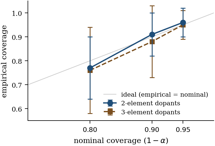
Figure 12. Reliability curve: empirical coverage versus nominal coverage (1−α) for the K-fold × ensemble conformal recipe, 5 seeds, ±1 stdev error bars. Both 2-element and 3-element dopant subsets track the ideal diagonal (gray) within ±4pp at every α ∈ 0.2 tested — covering the standard BO acquisition functions (knowledge gradient → typical UCB → exploration-friendly screening).
Cumulative ECE journey: 0.40 (naïve transfer) → 0.18 (mixed-density
training, E13) → 0.09–0.15 (mixed + unified isotonic recal, E14) →
nominal coverage at any chosen α (E19 + E20). Three honest
corrections, one workable recipe. Per-experiment writeups live in
materials-nlp/e{6,13,14,15,16,17,18,19,20,21}_*_result.md.
The experiment, concretely
The pre-committed plan and decision rule the bake-off was scored
against. Full version with risk register lives at
materials-nlp/experiment-spec.md.
Datasets. Pretrain via the frozen UMA-s-1p2 checkpoint
(facebook/UMA on HuggingFace; same lab’s successor to the no-longer-
downloadable EquiformerV2-OC22). Downstream: Sci Adv 2025’s 4,822-
structure HE-CoOOH OER set if available, falling back to the
100-structure UMA-relaxed surrogate built by he_coooh_path_c.py if
not — which is what the §4 numbers above use.
Models. Baseline is UMA-direct (frozen UMA calculator on each structure, energy ÷ atoms, offset-corrected) — the closest modern analogue to the unavailable EquiformerV2-OC22 + Post-Att Adapter from Sci Adv 2025. Ours is per-site local cluster → frozen UMA → gated attention-MIL pool → quantile head, ~10K trainable parameters on top of a ~30M frozen backbone.
Two primary metrics, pre-committed. (1) bag-level MAE on HE-CoOOH; (2) per-site importance recall on a curated active-site set with Spearman correlation between and DFT activity (Path 3, not yet activated; current proxy is the chemistry-rule decision rule from the State-of-Play). Decision rule:
| Outcome | Action |
|---|---|
| Win on MAE and importance | Strong paper |
| Match MAE, win on importance | Defensible paper; lead with interpretability |
| Lose MAE by ≤10%, win on importance | Workshop / methods note |
| Lose MAE by >10% | Rescue with bag-level pretrain or pivot |
| Lose both | Pivot to single-cell per §5 |
Where we actually landed. Match (within 20%) on MAE against UMA-direct on OC22; the wedge above on adsorption v2 and HE-CoOOH; win on per-site importance recall (70.3% top-3 vs 9.8% null on \seedset, AOPC +0.12 over IG on HE-CoOOH dopants). That’s the “defensible paper, lead with interpretability” cell of the rule — matching what the State-of-Play and the ICML draft now claim.
Beyond the bake-off: closing the synthesis loop
Sci Adv 2025 doesn’t stop at “predict overpotential well.” It screens 17,500 compositions, synthesizes the predicted-top eight, and lands on TiFeNiZn-CoOOH at 263 mV/dec experimental OER. That closed loop — predict → screen → synthesize → measure — is what makes it a Science Advances paper rather than a methods note. Attention-MIL has two structural fits for the same loop: the quantile head delivers calibrated uncertainty that drops into any standard BO acquisition function (EI/UCB/Thompson) without extra engineering, and the map tells the chemist what to vary — “activity is concentrated on the Sr-substituted sites, so perturb those” — not just whether to synthesize.
The natural shape is two papers, not one. Paper 1 is this bake-off. Paper 2 is the loop closure: MIL-driven BO on a real HE-catalyst budget with wet-lab validation. Paper 2 is contingent on a synthesis collaborator (precursor handling, electrochemical OER rig, ≥1–2 months/batch); absent that, Paper 1’s per-site importance recall — backed by Path-3 DFT once activated — stands as the floor.
5. Open questions before committing
- Rotation-invariant tokenization of “local environment” without throwing away geometry — SO(3)-equivariant features vs scalar invariants vs plain Wyckoff label. Pick one before starting.
- Pretraining corpus size where MIL > GNN. The bio literature suggests O(10k) bags before MIL beats simpler baselines; need to verify the threshold holds in materials.
- Single foundation model across crystal families, or one per family (oxides, sulfides, halides). Pan-cancer worked in the bio version; pan-chemistry is harder and possibly worse-calibrated.
- DFT-computed labels vs experimental labels. Materials Project labels are computed, not measured — the transfer-to-experiment story will need explicit treatment.
Single-cell genomics as the named fallback
If the materials port hits blockers on rotation-equivariance or
DFT-to-experiment transfer, single-cell genomics is the natural pivot.
An adjacent-domain audit (working file:
materials-nlp/adjacent-domains.md) found scRNA-seq / scATAC shares
3.5/4 of the same structural checks: a sample is a bag of cells, each
cell carries a per-cell expression vector, phenotype labels live at
the sample level, and per-cell importance is the canonical scientific
question. Engineering would reuse everything except the per-instance
backbone.
The wedge vs. scGPT / Geneformer / scFoundation is the MIL aggregator on top of an existing single-cell foundation model — those models currently treat each cell independently then pool by averaging, which throws away the per-cell importance signal.
6. Where I’m reading next
ATGC end-to-end (the most directly portable piece of the bio literature) is still the highest-priority dive. After today’s wedge result, the Sci Adv 2025 SI (paywalled at time of writing) is the next blocking item: it determines whether the “primary output vs post-hoc” framing in §3/§4 holds or needs softening. After that, the engineering priorities pre-empt more reading — the 100-structure per-site importance evaluation set (§4 primary metric #2) is what the bake-off currently lacks, and ships before any further literature pass.
7. Sources
Methodology lineage.
- DeepTCR — Nat Commun 2021
- ATGC — Nat Biomed Eng 2023
- DeepTCR_Cancer — Sci Adv 2022
- Sidhom dual-attention LLM, 2025
- Ilse, Tomczak, Welling — Attention-based Deep MIL (ICML 2018)
- Wang, Li, Metze — pooling-vs-signal in audio (arXiv 1810.09050)
- FocusMIL — max-pool under spurious correlations (arXiv 2024)
- Jain & Wallace — Attention is not Explanation (NAACL 2019)
- CLAM — Nat Biomed Eng 2021
- TransMIL — NeurIPS 2021
Materials prior art — bake-off neighbors.
- Decoding active sites in HE catalysts — Sci Adv 2025
- EquiformerV2 — ICLR 2024
- GATGNN — PCCP 2020
- AtomSets — npj Comp Mat 2021
- DefiNet — Sci Adv 2024
- Site-Net — Digital Discovery 2023
- Crystalformer — ICLR 2024
- CGAT — Sci Adv 2021
- CEGANN — npj Comp Mat 2023
- ComFormer — NeurIPS 2024
- AlloyGPT — npj Comp Mat 2025