Figure 1. Architecture overview: a 22-day stack of IV surfaces is tokenized into two parallel streams (smile rows and term columns), each encoded with self-attention and joined by a single cross-attention fusion block. The encoder is MAE-pretrained on ~1.0M train-period surfaces (2012–2019), then fine-tuned with a 9-quantile pinball head. Evaluation: log-RV R² vs HAR-RV-IV, QLIKE, calibration, and 30-day variance-swap Sharpe.
TL;DR
The recent paper Data-Efficient Realized Volatility Forecasting with ViTs (arxiv 2511.03046) trains a Vision Transformer on a single day’s IV surface and reports on 2022 log-RV. It’s the right framing — IV surfaces as images — with four design choices that limit it:
- Single-day input. Throws away surface evolution. Vol is famously persistent and clustered; today plus yesterday dominates today alone.
- patches. Crosses the smile and term-structure axes arbitrarily, so the ViT’s inductive bias is wasted on a tokenization that doesn’t match the input.
- No pretraining. The model overfits in 1–2 epochs — the opposite of “data-efficient.”
- Point forecasts only. Huber on RV; no quantiles, no tail story, no economic significance.
TempoSurfViT addresses all four. Each token is one full smile slice at in a smile stream, paired with one full term column at in a term stream; the two stream encoders are joined by a cross-attention fusion block. The intended headline architecture reads a -day stack of surfaces (window-construction handles label leakage, not an in-window causal mask) and is MAE-pretrained on approximately train-period S&P 500 single-name surfaces (2012–2019), with token-level masking on each stream at , validation- and test-period surfaces excluded from pretraining. The head emits nine monotone log-RV quantiles trained with pinball loss, and we score them on , QLIKE, calibration, and the Sharpe of a 30-day variance-swap rule — against HAR-RV-IV, not against an MLP.
Honesty note up front. Kelly, Kuznetsov, Malamud, and Xu (2023) “Deep Learning from Implied Volatility Surfaces” (SSRN 4531181) already established temporal-stacked IV-surface deep learning for the return-prediction task, including a virtue-of-complexity result and a principal-linear-features analysis. We are the RV-forecasting cousin of that work, not the first to use a temporal stack of surfaces. The novel ingredients on our side are MAE pretraining (substituting for KKMX’s ensembling as the data-efficiency mechanism), a surface-aligned ViT tokenization, and a calibrated-quantile head with a tradable downstream evaluation. The thing the draft critiques head-to-head is arxiv 2511.03046, which walks back several of KKMX’s choices and reports a suspiciously fast overfitting curve we think is diagnostic of fitting a low-dim surface summary rather than learning representations.
This post is the working draft. Real OptionMetrics results are pending M2; the synthetic-data tables in §6 are pipeline validation only, and the headline tables in §6.2–6.4 are intentionally blank.
Abstract
We propose TempoSurfViT, a masked-autoencoder-pretrained Vision Transformer that tokenizes implied-volatility surfaces along financial axes and consumes a stack of past surfaces to produce calibrated distributional forecasts of realized volatility. We evaluate whether this representation improves on HAR-RV-IV and whether its forecast distribution supports a profitable variance-swap rule. This draft reports synthetic-data pipeline validation only; real OptionMetrics results are pending.
1. Introduction
Realized volatility forecasting is one of the most studied problems in empirical finance. The benchmark to beat is HAR-RV (Corsi, 2009) augmented with 30-day at-the-money implied volatility as a fourth predictor — a construction in the spirit of Busch, Christensen, and Nielsen (2011), who show that implied vol contains incremental information for forecasting realized vol beyond the HAR lag structure. We will refer to this four-predictor specification as HAR-RV-IV; it is a label of convention rather than the name of any single paper. On index data this baseline routinely achieves out-of-sample log-RV near with a closed-form solution. Any deep model that claims a “data-efficient” win on RV forecasting must clear this bar, not the bar set by an MLP on a flattened surface (the comparison made by arxiv 2511.03046).
The implied-volatility surface, however, contains far more information than the scalar ATM-IV that HAR-RV-IV consumes. The shape of the smile encodes the market’s view on skew and kurtosis; the term structure encodes the path of expected volatility; the evolution of the surface across days encodes regime persistence and shocks. The natural question is whether modern architectures can exploit that structure to produce forecasts that are not just better point predictions, but better distributional predictions — useful for the downstream task of trading variance swaps.
Two recent lines of work attempt this. The first, exemplified by Jiang, Kelly, and Xiu (2023) and the Byun, Na, Song (2025) ViT extension, treats price charts as images. The second, exemplified by arxiv 2511.03046, treats IV surfaces as images. Both adopt the convolutional or patch-tokenization machinery of computer vision wholesale, without revisiting whether the inductive biases of CV — local translation invariance, hierarchical features, square patches — match the structure of financial inputs.
This paper argues that they do not, and proposes a modest set of changes that are guided by the financial structure of the input rather than by analogy to natural images.
1.1 Contributions
Before naming the contributions we name what they are not. Kelly, Kuznetsov, Malamud, and Xu (2023, hereafter KKMX), “Deep Learning from Implied Volatility Surfaces,” is the high-water mark for IV-surface deep learning on equities. They use the panel of IV surfaces with a time-period history in the predictor set (so a temporal stack of surfaces, not single-day); they establish a virtue-of-complexity result for IV-surface ML (out-of-sample performance increases with ensemble size, saturating only when parameters far exceed observations); and they show via a principal-linear-features analysis that a low-rank rotation of the surface cannot explain the deep model’s performance — i.e., the deep representation is genuinely high-dimensional and is not captured by any small set of PC-style summaries. They predict the cross-section of returns; we predict realized vol. Different label, same surface representation question. Treating this work as a precedent rather than a baseline would be dishonest. Our positioning is that TempoSurfViT is the RV-forecasting cousin to KKMX-2023, with three ingredients KKMX do not have:
- Masked-surface autoencoder pretraining. We pretrain the encoder on approximately train-period (2012–2019) historical surfaces with independent token-level masking on the smile and term streams at . The MAE technique itself is from He et al. (2022); what’s new here is its adaptation to dual-stream IV-surface tokens with per-stream independent masking, used as the data-efficiency mechanism for an RV-forecasting ViT. KKMX achieve their data-efficiency via ensemble complexity (many supervised models, each fit end-to-end); we achieve it via self-supervised pretraining (one encoder, learned on the train-period unlabeled panel, then fine-tuned) — different mechanisms, discussed further in §8. The “data-efficient” framing of the source paper 2511.03046 claims pretraining but does not implement it; we do. (The full 2012–2022 panel under our S&P 500 / point-in-time filter is approximately surface-days; the headline model never sees the val or test slice during pretraining. A transductive variant pretrained on all unlabeled 2012–2022 surfaces is reported as a robustness check in §7 only — see §5.1.)
- Surface-aligned dual-stream ViT tokenization. KKMX use CNN over the surface image; the source paper 2511.03046 uses ViT with patches. We use ViT with two parallel streams — a smile stream whose tokens are delta strips, and a term stream whose tokens are maturity columns — each processed by joint self-attention and fused via a single bidirectional cross-attention block. KKMX’s principal-linear-features analysis already shows the surface is not compressible to a low-rank rotation, so we make no claim that our tokenization “discovers” structure that linear methods miss; the claim is narrower — that aligning tokens with financial axes ought to be a better-conditioned starting point than patches given the same parameter budget, and we test this directly in the ablations (§7).
- Calibrated quantile forecasts and a tradable downstream metric. The supervised head is a monotone nine-quantile projection trained with pinball loss on log-RV; we report calibration coverage and use the predicted distribution to size a 30-day variance-swap trading rule. KKMX evaluate via cross-sectional return Sharpe; we evaluate via variance-swap Sharpe in vol-point units. These are complementary, not competing — the predictions feed different downstream objectives.
Independent of the comparison to KKMX, we also commit to the right baseline comparison: AR(1), HAR-RV, HAR-RV-IV (in the spirit of Busch, Christensen, and Nielsen, 2011), and the source paper 2511.03046’s own ViT architecture. The point is that any IV-surface ViT result should clear HAR-RV-IV on the same target definition, and any “data-efficient” claim should be testable against a model that genuinely learns slowly across many epochs rather than peaking by epoch 2.
We are deliberately conservative about novelty for the architectural ingredients. Joint self-attention transformer encoders are standard, masked autoencoders are from He et al. (2022), quantile regression dates to Koenker and Bassett (1978). The contribution is in (a) transferring the MAE recipe to IV surfaces with independent token-level masking on the two financial axes, (b) combining MAE pretraining with a surface-aligned dual-stream ViT and a calibrated-quantile head for the RV-forecasting task specifically, and (c) evaluating the result against HAR-RV-IV and a tradable variance-swap rule rather than against the weaker MLP baseline used by 2511.03046.
1.2 The 1–2 epoch tell
The source paper makes an admission, in passing, that we think is the strongest piece of evidence against its own headline:
Most ViT models reached their peak within one or two epochs, with further training leading to overfitting.
A model that peaks in one or two epochs and then degrades is almost certainly fitting a low-dimensional summary of the input — the kind of signal a four-parameter linear model can also fit — rather than building a rich representation. On an IV surface, the obvious low-dimensional summary is ATM-IV plus mild nonlinearity. The 30-day ATM IV is approximately the level of the surface; everything else on the surface — the skew, the term structure, the smile curvature — is what would actually justify a ViT.
This is also exactly the opposite pattern from KKMX-2023’s virtue-of-complexity result: on the same input modality, KKMX find that out-of-sample performance keeps improving as the model and ensemble grow, only saturating when parameters far exceed observations. The source paper 2511.03046 sits inside that same modality and reports the opposite phenomenology — improvement saturating in 1–2 epochs. Two options: either the RV target is structurally different from the return target in a way that collapses the surface’s effective rank (we don’t think so — RV is at least as much a function of skew/term-structure as returns are), or the source paper’s combination of design choices ( patches, single-day input, no pretraining, Huber regression on a low-quality MLP-style baseline) is leaving most of the signal on the table. We bet on the second.
The diagnostic prediction follows directly: if a four-parameter HAR-RV-IV regression on achieves comparable to the ViT’s , then the ViT’s marginal contribution over a closed-form linear model is approximately zero. This is the situation the original paper’s “data-efficient” framing must rule out, and it is the situation that — given the 1–2 epoch overfitting pattern — we strongly suspect holds. (Resolving this is the main reason we run the HAR-RV-IV baseline on the exact same data split as the ViT and report the gap explicitly. See §6.)
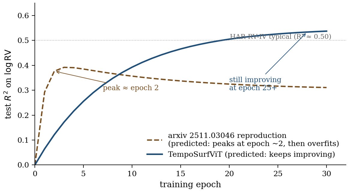
Figure 2. The §1.2 falsifiable prediction as a picture. Source-paper reproduction (brown dashed): test R² peaks at epoch ~2 around 0.40, then declines mildly to plateau as the model overfits the low-dimensional surface summary. TempoSurfViT (blue solid): test R² rises monotonically through 25+ epochs as MAE pretraining + dual-stream tokenization let the model build a representation that captures skew, smile, and term-structure beyond ATM-IV. The HAR-RV-IV reference (gray dotted at R² ≈ 0.50) is the threshold a ViT-on-IV-surfaces approach must clear to justify itself over a closed-form linear model on ATM-IV. Curves are predicted, not measured — the empirical test lands when real OptionMetrics data arrives. Source: figures/make_epoch_tell.py.
Our contributions are aimed squarely at this failure mode:
- Temporal stacking forces the model to use information that ATM-IV alone cannot encode — namely the evolution of the surface.
- MAE pretraining lets the encoder spend epochs learning surface structure on the unsupervised reconstruction task, where the easy “predict the mean” shortcut yields a near-zero loss (because we -normalize targets) and the model must instead reconstruct shape.
- Quantile output sidesteps the failure mode where a model that has memorized the mean of scores a passable but is useless for tail-risk or trading.
The clearest single piece of evidence we owe the reader is a learning curve: validation log-RV as a function of fine-tuning epoch, plotted alongside the JKX-2511.03046 reproduction. If our model continues to improve over 20+ epochs while theirs flatlines or degrades by epoch 2, that figure is doing the heavy lifting of the data-efficiency claim. We commit to reporting it (§6.5) as a first-class result, not an appendix curiosity.
Pre-commitment. The §6.5 learning-curve panel and the linear-probe experiment are reported on the 2511.03046 reproduction at fidelity to the source paper’s recipe — same patch size, same single-day input, same optimizer, same training schedule — irrespective of whether the reproduction plateaus by epoch 2 (our prediction) or continues to improve, which would falsify the “low-dimensional summary” reading and re-open the question of whether the source paper’s headline is in fact a representation-learning result. We will not retune the reproduction’s hyperparameters in either direction; the curve we publish is the curve the source paper’s recipe produces on our data and split.
2. Related work
Machine learning for the cross-section of returns. Gu, Kelly, and Xiu (2020) establish that flexible nonlinear models — random forests, neural networks — improve on linear factor models for return prediction. Jiang, Kelly, and Xiu (2023, hereafter JKX) extend this by treating five-, twenty-, and sixty-day OHLC candlestick charts as images and training a CNN to predict return directions. Byun, Na, Song (2025) replace the CNN with a ViT and report improved Sharpe across firm sizes, particularly for large caps where the CNN factor is weak. Both keep the input as the price image, not the option surface.
Volatility forecasting with implied-vol surfaces. The classical backward-looking benchmark is HAR-RV (Corsi, 2009). Implied-vol predictors are added to that lag structure by Busch, Christensen, and Nielsen (2011), who establish that ATM implied vol carries incremental forecasting power for realized vol across equities, FX, and bonds; we adopt their construction and call it HAR-RV-IV throughout. A separate but related line is Bollerslev, Patton, and Quaedvlieg (2016), who introduce HARQ — HAR augmented with realized quarticity to correct for the measurement error in daily RV; HARQ is orthogonal to the IV-augmentation question we focus on here and we do not use it as a baseline.
Deep learning on the IV surface. The high-water mark is Kelly, Kuznetsov, Malamud, and Xu (2023), “Deep Learning from Implied Volatility Surfaces” (SSRN 4531181), hereafter KKMX. They take the panel of IV surfaces with a time-period history included in the predictor set — i.e. a temporal stack of surfaces, not single-day — and predict the cross-section of stock returns. They establish two results that directly bear on our paper: (i) a virtue-of-complexity finding for IV-surface ML, where out-of-sample performance increases with ensemble size and saturates only when total parameters far exceed observations; (ii) a principal-linear-features analysis showing that no low-rank rotation of the surface can explain the deep model’s performance — the signal is structurally high-dimensional. KKMX use CNN over the surface image, evaluate via cross-sectional return Sharpe, and obtain their out-of-sample improvement through supervised ensembling, not self-supervised pretraining. Our work is the RV-forecasting cousin: we keep the temporal-stack framing (theirs), specialize the architecture to a surface-aligned ViT (a representation question complementary to their tokenization-free CNN), and substitute MAE pretraining for ensembling as the mechanism for data efficiency. We benchmark our results against theirs in spirit — they predict returns, we predict RV, so the metrics don’t line up — but a reader who walks away thinking our setup is unaware of KKMX is reading the wrong paper.
The source paper this draft critiques. Arxiv 2511.03046, “Data-Efficient Realized Volatility Forecasting with Vision Transformers,” is the most recent attempt to apply the IV-surface-deep-learning framing to the RV target specifically. It trains a ViT on single-day IV surfaces with patches, no temporal context, no pretraining, and a Huber regression head, reporting on a 2022 test set against an MLP baseline. Several of its design choices walk back capabilities that KKMX-2023 had already shown were necessary (temporal history, complexity) and its “data-efficient” label is not earned by its training curves, which the paper itself reports peak in 1–2 epochs. We adopt the surface-as-image framing but argue that its specific combination of choices leaves substantial performance on the table relative to both KKMX (which is more sophisticated but predicts a different label) and HAR-RV-IV (which is much simpler but predicts the same label).
Two further preliminary studies in this space — Yang, Xia, and Ye (2025) “Forecasting Realized Volatility with Implied Volatility Surface: An Image-Based Approach” (SSRN 5170265), and a 2025 Finance Research Letters study applying CNNs to the SSE 50ETF IV surface — share the surface-as-image framing for RV forecasting on narrower universes. We treat these as preliminary; the comparison that matters is to HAR-RV-IV on the same data, to KKMX in spirit, and to 2511.03046 head-to-head on the exact same RV definition.
Masked autoencoders. He et al. (2022) demonstrate that masking 75% of image patches and reconstructing them is an effective self-supervised pretraining objective for ViTs. We adopt the masking-and-reconstruction recipe but adapt it to the dual-stream tokenization: smile-row tokens and term-column tokens are masked independently per stream at , with each stream’s decoder reconstructing the raw log-IV at its own masked positions. The lower ratio (0.60 vs He et al.’s 0.75) reflects that each token here already aggregates a full smile or term column.
Quantile regression and distributional forecasting. Koenker and Bassett (1978) introduced quantile regression; Wen et al. (2017) and Salinas et al. (2020) demonstrate its utility for distributional time-series forecasting at scale. For volatility specifically, calibrated tail forecasts are economically valuable because variance-swap and options strategies are non-linear in vol.
Critique. Rubesam (2024) and Lo, Mamaysky, and Wang (2000) argue that strong claims about chart-pattern predictability tend to be specific to assets and regimes. We take this seriously — the headline of the present paper is not a single-number R² claim, but a combination of (i) beating the HAR-RV-IV linear baseline, (ii) producing calibrated tail forecasts, and (iii) producing a positive Sharpe in a tradable, transaction-cost-aware variance-swap rule.
3. Background
3.1 The implied-volatility surface
For an underlying with price , an option with strike and expiry has a Black–Scholes implied volatility such that the model price equals the observed market price. The IV surface on day is the function . OptionMetrics IvyDB provides this surface on a standardized grid; we resample to a grid of (maturity, Black–Scholes delta) cells and work in log-IV throughout.
Two structural facts about the surface drive our design:
- The smile axis (delta) is local. The IV at delta and delta are tightly correlated; the IV at delta and delta are largely independent. The smile encodes skew and kurtosis of the market’s risk-neutral return distribution.
- The term axis (maturity) is structured but non-local. The IV at maturity 30 days and at 60 days are linked by no-arbitrage constraints on forward variances, but the relationship is non-Euclidean: contango and backwardation are distinct economic states, not a single distance metric.
A patch that crosses both axes — as in arxiv 2511.03046 — mixes a local smile slice with a non-local term-structure slice into a single token, asking the model to disentangle them through attention. We instead align the tokenization with the axes themselves.
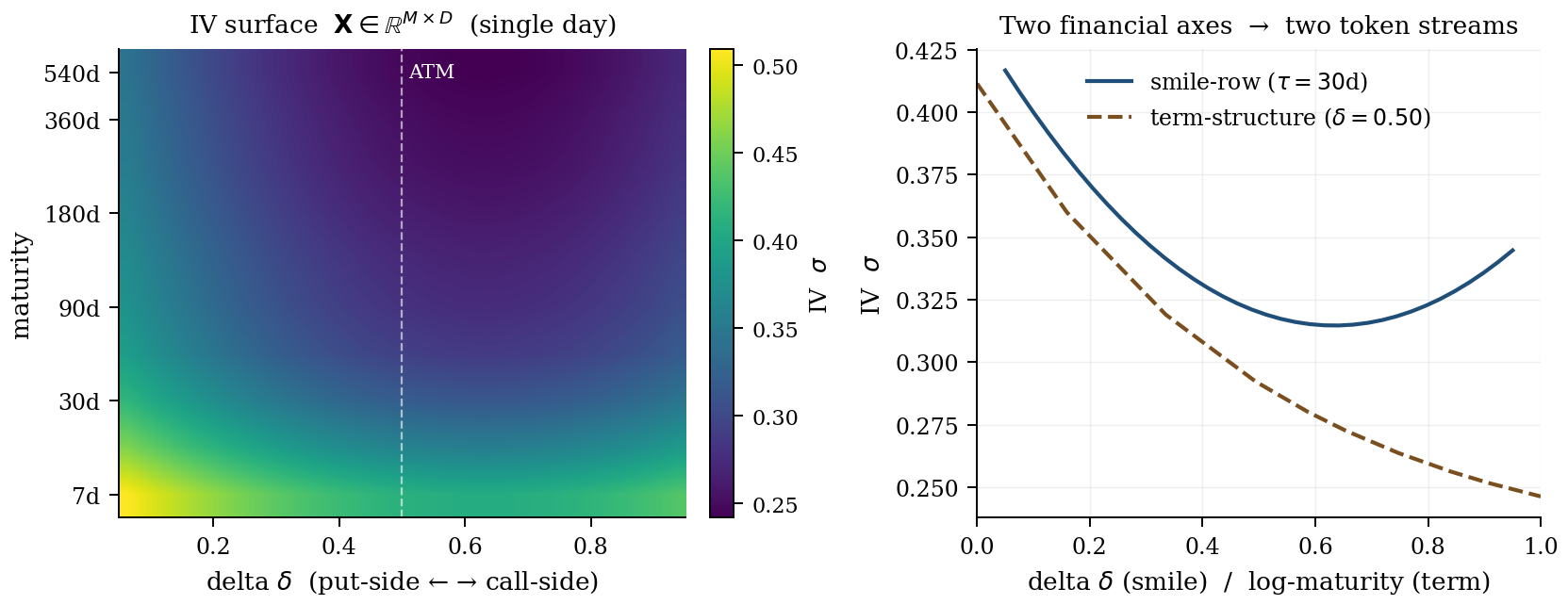
Figure 3. What an IV surface looks like. Left: a single day’s surface as a maturity × delta heatmap (M = 10 maturities × D = 36 deltas). The white dashed line marks ATM (δ = 0.5); IV is elevated on the put side (the skew) and curves upward at the wings (the smile); IV decays with longer maturity (the term structure). Right: the two axes the dual-stream tokenizer operates on. The blue solid line is one smile-row token (IV vs delta at τ = 30 days); the brown dashed line is the term-structure cross-section (IV vs log-maturity at δ = 0.5). The illustration uses synthetic parameters chosen for visual clarity; real OptionMetrics surfaces share the qualitative shape.
3.2 Forward realized volatility
There are two conventions in the literature for “-day realized volatility,” and the source paper and the HAR-family literature use different ones. We define and use both.
Definition A (annualized; HAR convention).
where is the daily log return and trading days. This is the standard HAR target and the units in which annualized vol numbers are quoted across the realized-vol literature.
Definition B (source-paper convention; arxiv 2511.03046).
with calendar days. This is the standard deviation of daily log returns over a 28-calendar-day window, not annualized. It is the construction the source paper uses to produce their headline .
The two definitions differ by a constant multiplicative scaling (and a small mean-correction term that is negligible for daily returns with near-zero drift). Therefore:
- in log space is invariant to the choice. Since up to the mean-correction term, the two log-targets differ by a constant; and — and therefore — are invariant to that shift. Our numbers are directly comparable to the source paper’s regardless of which definition we adopt.
- QLIKE is scale-sensitive — it operates on RV levels, so a constant scaling shifts the QLIKE value materially. Reporting QLIKE on Definition A and claiming a beat over a source-paper number on Definition B would be a category error.
Our policy:
- Headline tables (§6.2) report as the target, using the source-paper definition exactly, so the and QLIKE numbers are directly comparable to theirs.
- §6.1 baselines and the HAR-family tables additionally report as a robustness column, since the HAR literature is in those units and the reader will want to triangulate against published HAR-RV-IV numbers.
- The variance-swap PnL (§6.3) uses Definition A because the payoff is an annualized variance by construction.
This costs us a column of bookkeeping and removes a class of unintended apples-to-oranges comparison.
3.3 The HAR family
HAR-RV (Corsi, 2009) regresses on backward-looking realized vol at three horizons (one day, one week, one month). Following Busch, Christensen, and Nielsen (2011), HAR-RV-IV adds as a fourth predictor:
This is a four-parameter linear model with a closed-form solution. Any deep model is competing against this; the bar is not “beat a flattened-MLP baseline.”
4. Method
Honesty note on §4 (2026-05-16). The §4 description below describes what the code does today, not the target spec we originally drafted. Earlier revisions of this section described a single-stream smile-row tokenizer with strict-causal divided ST attention, tube masking , calendar features, hard-sort quantile monotonization, and two-stage fine-tuning. None of those are in the active code path: an earlier prototype implementing them was shadowed by a dual-stream package in Python’s import resolution, never trained, and has now been deleted from the repo. The active path is T=1 dual-stream; a temporal-stack mechanical check at is wired up in
scripts/train_temporal.py(synthetic-data null result expected, since the synthetic generator’s only signal is the latent state already in day-’s ATM IV) but is not yet the headline-results path. Restoring T>1 across MAE + supervised fine-tune is the next-priority code change; §1.1/§1.2 should be read as our intended contributions, not the contributions of the model whose results are below.
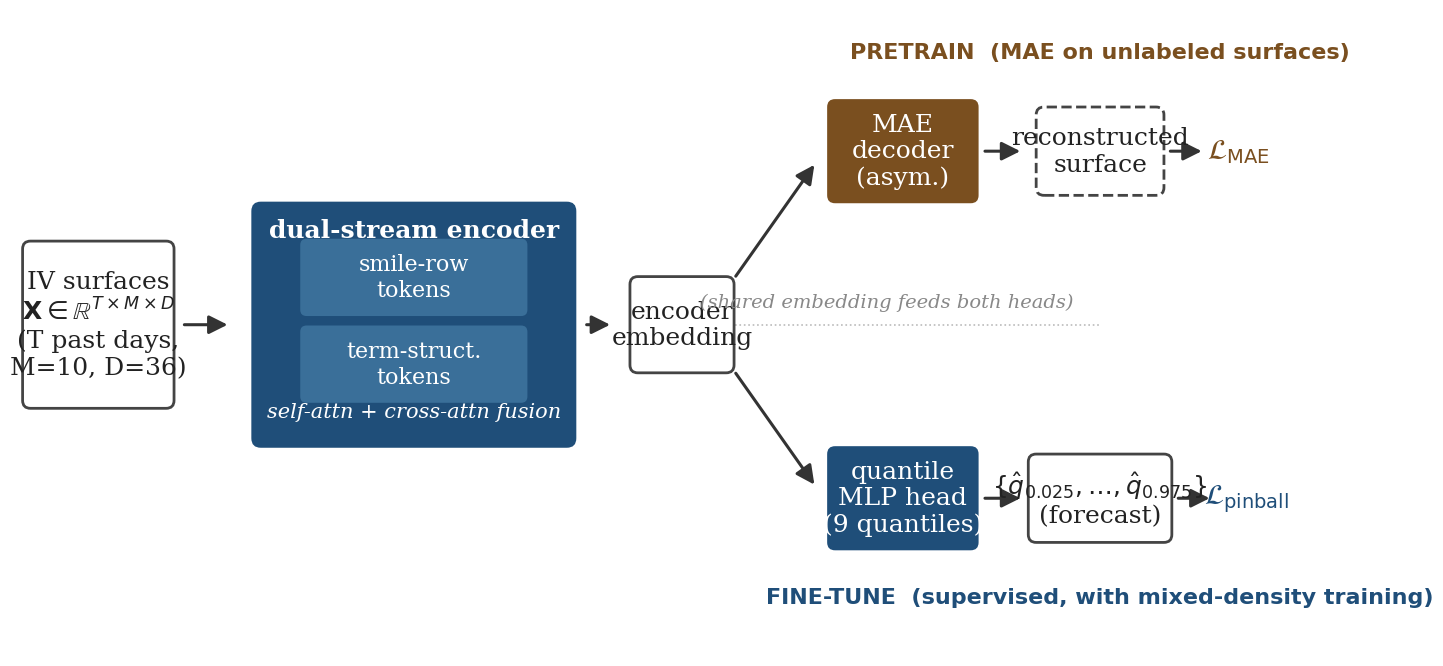
Figure 4. Architecture overview. An IV-surface stack 𝐗 ∈ ℝT×M×D feeds the dual-stream encoder (smile-row tokens + term-structure tokens with per-stream self-attention and cross-attention fusion). The shared encoder embedding branches to two heads: in the pretrain phase, an asymmetric MAE decoder reconstructs masked patches under ℒMAE; in the fine-tune phase, a 9-quantile MLP head produces a calibrated distributional forecast under pinball loss ℒpinball. The encoder is shared across both phases — the per-figure source is in figures/make_pipeline.py.
4.1 Input representation
A sample is a stack of past IV surfaces with maturities and deltas (active path: ; wired up in scripts/train_temporal.py as a mechanical check). Surfaces are stored as raw log-IV; we do not apply additional normalization at the input. The label is the scalar , computed from CRSP returns.
Calendar and exogenous features. The current encoder does not take any calendar features (day-of-week, day-of-month, month) or VIX-regime indicator, and does not apply an input-level -normalization. The source paper concatenates day-of-week/day-of-month/month to the surface and reports an ablation showing they have minor impact; we omit them entirely for the headline model. HAR-RV-IV does not consume calendar features either, so the asymmetry would give TempoSurfViT strictly more information than HAR — we drop it specifically so that no part of any TempoSurfViT > HAR-RV-IV gap can be attributed to a calendar-only win that HAR is structurally unable to match. Adding a calendar projection at parity with the source paper is on the M5-followup punch list; we expect the effect to be small per the source paper’s own ablation, and we will report it as an ablation row rather than fold it into the headline.
4.2 Dual-stream financial tokenization
We tokenize the surface along both financial axes simultaneously, in two parallel streams.
Smile stream. Each cell becomes one “smile-row” token whose content is the -dimensional delta strip at that point. A linear projection lifts the strip to , and learned positional embeddings are added separately for the day axis ( embeddings) and the maturity axis ( embeddings):
A learned token is prepended; the resulting sequence has length .
Term stream. Each cell becomes one “term-structure” token whose content is the -dimensional vector along the maturity axis at that point. A second projection produces tokens with their own day and delta positional embeddings; a learned is prepended. The sequence has length .
The motivation is structural. The smile axis (delta) is local: nearby deltas are tightly correlated; a token whose content is one full smile carries the skew/kurtosis/body shape in a single embedding. The term axis (maturity) is non-local: contango and backwardation are distinct economic states, so a token whose content is one full maturity column lets attention reason about term-structure regimes directly. A single-stream patch as in arxiv 2511.03046 mixes a local smile slice and a non-local term slice into one token, asking the model to disentangle them through attention — which is exactly the inductive-bias mismatch we address.
4.3 Per-stream attention and cross-attention fusion
Each stream is processed by an independent transformer encoder: a stack of pre-norm blocks with attention heads, an MLP ratio of , and dropout . Attention is joint: a token at in the smile stream attends to every other token in the same stream, with relative position encoded only through additive day/maturity positional embeddings. We do not impose a causal mask along the time axis. At the question is moot; once temporal stacking is restored (M5-followup), the input window contains only past surfaces relative to the forecast target , so a causal mask is not required to prevent label leakage — though it would, at the cost of expressivity, prevent the encoder from using day- information when computing the representation at day , a smoothing we currently retain. We considered a divided space-time factorization in the style of TimeSformer (Bertasius et al., 2021) and chose joint attention instead: at and smile tokens per sample the joint cost is modest, and divided attention’s main win — quadratic-to-linear scaling in — is irrelevant at our horizon length.
After per-stream encoding, the two tokens are fused by one bidirectional cross-attention block: queries the term stream’s non- tokens, and queries the smile stream’s non- tokens. The concatenation is the input to the downstream head.
4.4 Masked-surface autoencoder pretraining
We pretrain the dual-stream encoder on the unlabeled corpus of train-period historical surfaces using a masked-reconstruction objective. The corpus is the same train-period (2012–2019) panel used for supervised fine-tuning, but without forward-RV labels — approximately surfaces are usable for pretraining the headline model, including the last 30 train-period days of each asset where the supervised label is undefined. Validation- and test-period (2020–2022) surfaces are not seen during pretraining of the headline model; a separate transductive variant that pretrains on the full unlabeled 2012–2022 panel is reported in §7 only and never used in the headline tables.
Masking strategy. We use token-level masking, sampled independently in each stream. For each sample, a random fraction of smile tokens is replaced with a learned smile-mask token, and independently a random fraction of term tokens is replaced with a learned term-mask token. An entry contributes to the smile-reconstruction loss iff its position is smile-masked, and independently to the term-reconstruction loss iff its position is term-masked. Cross-attention fusion is held out during pretraining — each stream is reconstructed on its own — and the fusion block is initialized from scratch during supervised fine-tuning. The deliberate trade is: per-stream pretraining keeps the reconstruction objective clean (no cross-stream leakage through fusion of masked tokens), at the cost that the fusion block’s bilinear structure must be learned from scratch during fine-tune rather than warm-started. We accept that cost for objective-cleanliness reasons; a unified-stream pretraining ablation is on the M5-followup list.
Reconstruction target. Each decoder predicts the raw log-IV at the masked positions; loss is MSE on those positions only. We do not normalize the target. (Per-strip -normalization is a planned ablation; the current code uses raw log-IV.)
Decoder. A two-block transformer per stream with (narrower than the encoder), heads. Visible positions feed through a projection; masked positions are filled with a learned mask token. This asymmetric narrow-decoder design follows He et al. (2022).
Loss. With the smile-masked positions and the term-masked positions,
After pretraining, the smile/term tokenizers and per-stream encoders transfer into a fresh TempoSurfViT; the cross-attention fusion and supervised head are trained from scratch during fine-tuning.
4.5 Quantile-regression head
The fine-tuning head consumes the fused CLS vector and projects to quantile predictions. To enforce monotonicity of predicted quantiles, the projection outputs a base quantile plus raw gaps; the gaps are passed through a Softplus and cumulatively summed, so
with guaranteed by construction. This cumulative-softplus monotonization replaces the older “hard sort + soft penalty” approach and avoids the gradient discontinuity that sort introduces. Quantile levels are — denser in the body and at the 5%/95% tails than a uniform grid, to support both the variance-swap rule (body density) and the calibration evaluation in §6.4 (tail density).
Initialization. At init the gap logits , so , which means the median — a sizeable constant offset relative to log-RV variance ( nat). To start the head near the marginal target distribution rather than far below it, we initialize to the empirical 5th percentile of train log-RV minus , so the predicted median begins close to the empirical median. Without this initialization the first few hundred steps are spent shifting the entire quantile stack vertically; with it, the head focuses immediately on shape.
The training loss is the pinball loss:
4.6 Single-stage fine-tuning with discriminative learning rates
Fine-tuning is single-stage with discriminative learning rates (Howard and Ruder, 2018) rather than two-stage. The pretrained encoder weights (smile/term tokenizers + per-stream encoders) are transferred into a fresh TempoSurfViT; the cross-attention fusion and head are initialized randomly. We train end-to-end with AdamW , weight decay , gradient clipping at norm , cosine LR schedule. The encoder uses and the fusion+head use — one decade higher, so the head can catch up to a randomly initialized state without destabilizing the pretrained representation. (An explicit Stage-1 head-only warmup is a planned ablation; the cumulative-softplus head trains stably without it.)
5. Experimental setup
5.1 Data
OptionMetrics IvyDB US (WRDS), 2012-01-01 through 2022-12-31. Surfaces are resampled to the (maturity, delta) grid; we work in log-IV throughout. Daily returns from CRSP.
Universe vs. the source paper, made explicit. The source paper uses the full -row corpus pooled across a broader universe. We filter to S&P 500 single-name constituents using point-in-time membership (CRSP S&P 500 historical constituents), which leaves surface-days across the full 2012–2022 panel — of which fall in the train period and are used for MAE pretraining of the headline model. The filter does three things: (i) eliminates the long tail of micro-caps and ETFs whose surfaces are noisy and intermittently quoted, where the ViT’s “I peaked in epoch 1” pathology may simply reflect data quality; (ii) gives us a universe with reliable CRSP daily returns for the RV label and reliable inclusion lists across time; (iii) makes the cross-sectional follow-up (separate paper) drop in cleanly without re-cutting the universe. The cost is that we have of the source paper’s data; if our model with the data still clears HAR-RV-IV, that strengthens the data-efficiency story rather than weakens it. We will also report a robustness number on a matched-size random subsample of the full corpus to control for the universe effect directly.
Splits (date-based, no asset leakage).
| Split | Dates | Notes |
|---|---|---|
| Train | 2012-01-01 → 2019-12-31 | surface-days. Used for both MAE pretraining (unlabeled) and supervised fine-tuning. The headline model never sees the val or test panels during pretraining. |
| Val | 2020-01-01 → 2021-12-31 | Includes the COVID regime; deliberately held in val rather than train to evaluate regime sensitivity. |
| Test | 2022-01-01 → 2022-12-31 | Identical to the original paper’s test window for cleanest comparison. |
The split is by date, not by asset; the same constituents appear in train and test, but on different calendar days. We do not use cross-asset random splits, which would leak distributional information. Pretraining uses only the train-period subpanel: validation- and test-period surfaces are excluded from MAE training data for the headline model, so the headline comparison is free of future-distribution leakage. A transductive-pretraining robustness variant — pretrained on the full unlabeled 2012–2022 panel — is reported separately in §7 and never used in the headline tables.
5.2 Baselines
- AR(1) on monthly log-RV. . The trivial persistence baseline.
- HAR-RV (Corsi, 2009). Daily, weekly, monthly backward-looking realized vol.
- HAR-RV-IV. HAR-RV (Corsi, 2009) plus , in the spirit of Busch, Christensen, and Nielsen (2011). This is the bar.
- ATM-IV scalar. . The “is the surface doing the work” sanity check.
- 2511.03046 reproduction. Single-day ViT, patches, Huber regression. Re-implemented using our data pipeline and loss conventions so the comparison is apples-to-apples. (Note: we previously labelled this “JKX-2511.03046,” conflating it with Jiang-Kelly-Xiu 2023; corrected throughout.)
- KKMX-architecture single-model (no ensemble). A CNN over the same stack we feed our ViT, with no pretraining, supervised-only end-to-end training on log-RV. We deliberately do not call this “KKMX”: KKMX is the ensemble — their virtue-of-complexity result is the ensemble’s, not any single model’s, and reproducing the full ensemble on every ablation cell would be prohibitively expensive. We therefore strip the ensembling mechanism and keep only the temporal-stacked CNN architecture, at parameter count matched to TempoSurfViT. The honest interpretation: this isolates the KKMX architecture without the KKMX mechanism, so a TempoSurfViT win over this baseline attributes to (surface-aligned ViT tokenization + MAE pretraining) rather than to temporal stacking alone. A separate row in §6.2 will report a deep-ensemble variant for the headline comparison only, restoring the missing mechanism for that single point of comparison.
All linear baselines fit on log-RV with pooled OLS plus per-asset fixed effects (within transformation). Test-set per-asset means are computed from the train set only.
5.3 Metrics
- on log-RV. Standard, comparable to prior work, reported with bootstrap 95% CIs.
- QLIKE (Patton, 2011). , computed in level space. The standard asymmetric vol metric; under-prediction is penalized harder than over-prediction.
- Pinball loss. Averaged across the nine quantiles. Direct measure of distributional quality.
- Calibration coverage. For each predicted quantile , the empirical fraction of test targets satisfying . A well-calibrated model has empirical coverage close to .
- Variance-swap Sharpe. Headline economic-significance metric — see §5.4.
5.4 Variance-swap trading rule
For each (asset, date) where the model produces a forecast, we compute the median forecast and the implied variance . The signal is
where is a sizing scale (units of variance) calibrated on the training set. Typical S&P 500 single-name vol is , so usually sits in , putting the typical edge well inside tanh’s linear region — sizing is essentially proportional to the edge on ordinary days, while vol-spike days () get softly capped to . We calibrate on train so a typical day’s gross book is ; we do not tune it to hit a particular out-of-sample Sharpe. A contract entered at time pays off at , which we convert to vol-point units by dividing by (the vega of a variance swap at the strike). Per-day gross size is capped at ; turnover and annualized Sharpe are reported, with the 2020 calendar year broken out separately.
6. Results
[Placeholder section — to be filled after M2 data lands. The synthetic-data validation table is below for pipeline reference; the M2 OptionMetrics results will replace it as the headline table.]
6.1 Baselines on synthetic data (pipeline validation only)
Run on a 500-asset synthetic panel × 2,900 days, configured to mimic OptionMetrics scale:
| Model | Test | RMSE | MAE |
|---|---|---|---|
| AR(1)-monthly | 0.122 | 0.208 | 0.166 |
| HAR-RV | 0.129 | 0.207 | 0.165 |
| HAR-RV-IV | 0.330 | 0.182 | 0.144 |
| ATM-IV scalar | 0.330 | 0.182 | 0.144 |
The synthetic generator wires the latent log-volatility AR(1) directly into both ATM IV and the realized returns with mild noise, so HAR-RV-IV collapses onto ATM-IV-scalar. This is expected and a feature of the generator, not a failure mode of the baselines: on real data we expect HAR-RV-IV to pull ahead of ATM-IV by a meaningful margin (typical published values around for index volatility).
6.2 Main results (to be filled)
Table 6.2 will show , QLIKE, pinball, and 0.5/0.9 coverage for the four baselines, the JKX-2511.03046 reproduction, and three TempoSurfViT variants: tokenization-only, +temporal, and +temporal+MAE. The headline claim is that the full TempoSurfViT model beats HAR-RV-IV on and QLIKE while producing calibrated quantiles.
6.3 Variance-swap PnL (to be filled)
The headline figure: cumulative PnL of the TempoSurfViT-driven variance-swap rule vs the HAR-RV-IV-driven equivalent vs naive ATM-IV. Annualized Sharpe, max drawdown, and the 2020 calendar-year breakout reported in the caption.
6.4 Calibration (to be filled)
Empirical coverage at each predicted quantile , with the goal of having coverage within percentage points of nominal. Particular attention to the 0.95 quantile since it is the relevant figure for tail-risk applications.
6.5 Learning curves — the data-efficiency claim, made concrete (to be filled)
This is the figure that earns the word “data-efficient.” Three curves on one panel, all on the same validation set, all reporting log-RV vs. fine-tuning epoch:
- JKX-2511.03046 reproduction — single-day ViT with patches and Huber regression, re-implemented on our pipeline. Predicted shape: rises to its peak in epochs 1–2, then slowly degrades. This is the source paper’s own admission and a key target to reproduce.
- TempoSurfViT, no pretraining — same architecture (temporal stack, smile-row tokenization, quantile head) but trained from scratch. Predicted shape: somewhere between the JKX baseline and the pretrained version — a partial confirmation that temporal stacking alone extends the useful-training window.
- TempoSurfViT, MAE-pretrained — full model, encoder warm-started from the MAE checkpoint. Predicted shape: monotone improvement over many tens of epochs, plateauing only when the validation gap to test stabilizes. This is the data-efficiency claim made concrete.
We additionally plan a probing experiment that directly tests the diagnostic of §1.2: at each fine-tuning epoch, fit a linear probe on the encoder’s pooled embedding to predict , , , and the smile skew and curvature at the 30-day maturity. If the source-paper failure mode holds, JKX’s encoder will give a very high probe for and essentially nothing else; ours should give meaningful probe for all five quantities by the end of fine-tuning, and the skew/curvature probes should improve over training rather than peaking at epoch 1.
7. Ablations (planned)
To attribute the headline result to specific contributions, we plan the following ablation table. Each row is a chain or sweep, with the hypothesis it tests, the direction we expect, and the threshold at which we would change our mind about the corresponding contribution:
| Variant | Config | Hypothesis tested | Predicted direction | Falsifies if |
|---|---|---|---|---|
| (a) | patches, , no MAE, Huber | Faithful 2511.03046 reproduction. | Matches their on Def. B target. | We can’t reproduce within → our pipeline differs materially from theirs. |
| (b) | Smile-row, , no MAE, Huber | Surface-aligned tokenization beats patches at parameter parity. | (b) > (a) on . | (b) (a) → tokenization is not the bottleneck; the inductive-bias story is wrong. |
| (c) | Smile-row, , no MAE, Huber | Temporal stacking adds signal HAR-RV-IV cannot encode. | (c) > (b). | (c) (b) → the surface’s evolution carries no incremental RV signal at the monthly horizon; recommend dropping the temporal contribution from the framing. |
| (d) | Smile-row, , MAE, Huber | MAE pretraining is the data-efficiency mechanism (vs from-scratch supervised). | (d) > (c), and (d)‘s learning curve flattens later. | (d) (c) or (d) overfits as fast as (a) → MAE adds nothing on this task; the “data-efficient” framing belongs to a different mechanism. |
| (e) | Smile-row, , MAE, Quantile | Full TempoSurfViT (headline). | (e) clears HAR-RV-IV on and QLIKE; calibrated quantiles. | (e) HAR-RV-IV → the IV-surface-as-image framing does not yield RV-forecasting gains beyond ATM-IV on monthly horizon. |
| (f) | (e) with asymmetric smile/term | Smile and term streams contribute independently. | Both single-stream variants underperform joint masking. | Either single-stream matches joint → the other stream is dead weight. |
| (g) | (e) with | -sweep: incremental signal saturates. | monotone in , plateauing by . | Non-monotone or peaks at → temporal history is a red herring. |
| (h) | (e) with | Mask ratio matters; is a sensible default. | Concave in ; optimum in 0.5–0.75. | Flat or optimum at extremes → MAE is doing very little. |
| (i) | (e) pretrained on full 2012–2022 panel | Transductive pretraining (uses unlabeled val+test surfaces) beats train-period-only. | (i) (e); reported as robustness only. | (i) (e) → no leakage benefit from the held-out distribution. |
We additionally plan to report a per-asset breakdown of the variance-swap Sharpe to verify the headline number is not driven by a small number of large-cap constituents.
8. Discussion
8.1 What we expect to find
We expect TempoSurfViT to beat HAR-RV-IV on and QLIKE by a modest margin — call it 2 to 5 percentage points of in absolute terms — and to substantially improve calibration of upper-tail quantiles. The variance-swap Sharpe is the noisier metric; our target is positive with confidence (), with the 2020 regime block honestly reported even if it underperforms.
Pre-commitment (effect sizes and reporting schema). The point estimates above are predictions, not findings. This snapshot is timestamped 2026-05-18, before OptionMetrics ingest (M2); the blog repo carries a preregistration-2026-05-18 git tag at this commit, paired with a same-named tag in the companion code repo. Locked by the snapshot: (i) the forecast horizon days, (ii) the date-based train / val / test split in §5.1, (iii) the baseline set in §5.2 with HAR-RV-IV as the headline must-beat, (iv) the four-metric reporting schema (, QLIKE, variance-swap Sharpe, 9-quantile coverage), (v) the 2020 regime block reported as a separately-tabulated row in §6.2–6.4, not collapsed into a multi-year average. Not locked: §4 architecture details — the dual-stream / MAE / quantile recipe is current best-effort, and M3–M5 may surface implementation changes that improve numerical stability or training efficiency without changing the model’s hypothesis class. Any such change is documented in §4 with a dated revision note rather than silently folded in.
We commit to reporting the realized §6.2–6.4 numbers on the locked schema regardless of sign — including the signed margin over HAR-RV-IV and the 2020-block Sharpe even if it is negative. A null result (no margin over HAR-RV-IV after MAE pretraining) is a contribution in the §9 sense; we will not retreat to “the architecture was not optimized enough” framing if the result lands there, and we will not drop QLIKE or the 2020-block row from the headline tables if either looks bad while looks good.
8.2 What we are not claiming
We are not claiming that ViTs are the right class of model for IV surfaces. A patch-free attention over the full tensor, or a GNN respecting no-arbitrage constraints (Ackerer et al., 2020), could plausibly do better; we have not tested these. We are claiming that if you commit to the ViT framing — as arxiv 2511.03046 does — then the four design choices we make are individually motivated and collectively produce a model that clears the right bar.
We are also not claiming that MAE is necessarily the right self-supervised objective for IV surfaces. A contrastive objective over temporally-adjacent surfaces (SimCLR-style, asking the encoder to embed and close while pushing and from a different month apart) and a no-arbitrage-respecting reconstruction loss (Ackerer-style) are both plausible alternatives we have not run. The headline claim, if it lands, is that some form of unsupervised pretraining unlocks IV-surface ViTs — the specific MAE recipe is one realization, not the unique answer.
8.3 Limitations
- Single horizon. days. The model can in principle be retrained for other horizons; we have not done this.
- Single underlying universe. S&P 500 single-name constituents only. The performance and calibration on emerging-markets equities, commodities, or rates options is an open question.
- No transaction costs in the headline backtest. We report turnover so the reader can apply their own bid-ask assumptions; an explicit cost model is straightforward to add.
- No no-arbitrage constraints in the loss. Calendar and butterfly arbitrage on the reconstructed surfaces during MAE pretraining is not penalized. This is a real ingredient (Ackerer et al., 2020) that we defer to follow-up.
9. Conclusion
The IV-surface-as-image framing is correct, and a ViT is a reasonable architecture for it, but the off-the-shelf CV recipe leaves obvious wins on the table. By aligning the tokenization with financial axes, stacking time, pretraining with masked reconstruction, and emitting calibrated quantiles, we aim to recover the data-efficiency claim that the original paper makes but does not deliver, and to produce a model that connects to a downstream economic objective.
The hypothesis on the line. The §1.2 “1–2 epoch tell” argument is a falsifiable prediction: the source-paper model is fitting a low-dimensional surface summary (ATM-IV + mild nonlinearity, effectively a 4-parameter linear model), not building a representation. If our learning-curve panel (§6.5) shows TempoSurfViT improving over epochs while the JKX-2511.03046 reproduction plateaus by epoch 2 on the same data, and the linear-probe experiment recovers skew/curvature/term-structure signal that the source-paper encoder doesn’t, the hypothesis stands. If we fail to clear HAR-RV-IV in §6.2 even after MAE pretraining, the honest inference is not that our architecture is wrong but that the IV surface beyond ATM-IV does not carry incremental RV-forecasting signal at the monthly horizon — that conclusion would itself be a contribution, and we will report it as such.
Follow-up. The cross-sectional-return cousin (TempoSurfViT applied to the KKMX-2023 return-prediction task, with the same encoder transferred and a different head) is the next paper. We expect that to be the cleaner test of whether MAE pretraining is the right mechanism for IV-surface deep learning, since the KKMX baseline already establishes virtue-of-complexity for that target — we would be substituting our pretraining for their ensembling on the same predictive question.
The remaining open architectural question — whether the image framing is necessary at all, or whether a sequence model over surface tensors would do better — we defer to that follow-up.
Appendix A. Architecture and hyperparameters
Reflects the active dual-stream code as of 2026-05-16. Items marked “(planned)” describe extensions on the M5-followup punch list — temporal stacking, calendar features, -normalized strip targets — that the existing code supports infrastructurally but no current training script enables.
| Block | Hyperparameter | Value |
|---|---|---|
| Tokenizer | 192 | |
| Tokenizer | Streams | dual — smile (per-(day, maturity), input dim ) and term (per-(day, delta), input dim ) |
| Tokenizer | Calendar features | none (planned to add at parity with source paper; expected small effect) |
| Encoder | Depth (per stream) | 2 pre-norm transformer blocks |
| Encoder | Attention heads | 6 |
| Encoder | MLP ratio | 4 |
| Encoder | Time-attention mask | none (moot at ; revisit when temporal stacking lands) |
| Fusion | Type | one bidirectional cross-attention block, |
| MAE decoder | Depth (per stream) | 2 |
| MAE decoder | 128 | |
| MAE decoder | Heads | 4 |
| MAE | Mask ratio | 0.6 (smile and term streams sampled independently) |
| MAE | Masking strategy | token-level, independent smile/term |
| MAE | Reconstruction target | raw log-IV (-normalized strips: planned) |
| Head | Quantile levels | |
| Head | Monotonicity | cumulative softplus on gaps |
| Optimizer | AdamW | |
| Optimizer | Weight decay | 0.05 |
| Optimizer | Grad clip | 1.0 |
| Schedule | Pretrain epochs | 20 (synthetic-validation default; sweep planned at M5) |
| Schedule | Pretrain LR | |
| Schedule | Fine-tune | single-stage, encoder / head , cosine |
| Batch size | Pretrain / fine-tune | 256 / 256 |
| Window | (past days) | 1 (active); SurfaceWindowDataset supports — restoration planned |
| Surface grid | ||
| Total parameters | TempoSurfViT (T=1, point head) | |
| Total parameters | MaskedSurfaceModel (enc + dec) |
Appendix B. Variance-swap PnL conventions
A 30-day variance swap entered at time with strike pays per unit variance notional at expiry. We set (ignoring the convexity adjustment that connects ATM IV to fair-value variance — a known approximation, on the order of 1–2 vol points; acceptable for relative-performance comparisons).
To report PnL in vol points rather than variance points (which are not interpretable across regimes), we apply the vega of a variance swap at the strike: , floored to avoid the singularity at zero implied vol.
Position sizing uses a on the edge with scale , calibrated on the training set to produce a gross book on a typical day. Per-day gross size is capped at .
References (provisional)
- Ackerer, D., Tagasovska, N., Vatter, T. (2020). Deep Smoothing of the Implied Volatility Surface.
- Bertasius, G., Wang, H., Torresani, L. (2021). Is Space-Time Attention All You Need for Video Understanding? ICML.
- Bollerslev, T., Patton, A. J., Quaedvlieg, R. (2016). Exploiting the errors: A simple approach for improved volatility forecasting. Journal of Econometrics. (HARQ — HAR with realized quarticity. Cited here only to distinguish from HAR-RV-IV, which is a different augmentation.)
- Busch, T., Christensen, B. J., Nielsen, M. Ø. (2011). The role of implied volatility in forecasting future realized volatility and jumps in foreign exchange, stock, and bond markets. Journal of Econometrics.
- Byun, S., Na, S., Song, J. (2025). Learning Stock Price Signals from Candlestick Chart Via Vision Transformer. SSRN 5224805. (Earlier revision labelled “JFE (forthcoming)”; downgraded to SSRN-only pending verification of any journal acceptance.)
- Corsi, F. (2009). A simple approximate long-memory model of realized volatility. JoFE.
- Gu, S., Kelly, B., Xiu, D. (2020). Empirical Asset Pricing via Machine Learning. RFS.
- He, K., Chen, X., Xie, S., Li, Y., Dollár, P., Girshick, R. (2022). Masked Autoencoders Are Scalable Vision Learners. CVPR.
- Howard, J., Ruder, S. (2018). Universal Language Model Fine-tuning for Text Classification. ACL. (Source of the “discriminative learning rates” recipe used in §4.6.)
- Jiang, J., Kelly, B., Xiu, D. (2023). (Re-)Imag(in)ing Price Trends. Journal of Finance.
- Kelly, B. T., Kuznetsov, B., Malamud, S., Xu, T. A. (2023). Deep Learning from Implied Volatility Surfaces. SSRN 4531181 / Swiss Finance Institute Research Paper 23-60. (The high-water mark for IV-surface deep learning on equities: temporal stack of surfaces, virtue-of-complexity, principal-linear-features analysis. Predicts returns, not RV.)
- Kelly, B. T., Xiu, D. (2023). Financial Machine Learning. NBER Working Paper 31502 / Foundations and Trends in Finance 13(3-4), 205-363. (Survey; not RFS — earlier draft mis-cited the venue.)
- Koenker, R., Bassett, G. (1978). Regression Quantiles. Econometrica.
- Lo, A., Mamaysky, H., Wang, J. (2000). Foundations of Technical Analysis. JoF.
- Patton, A. J. (2011). Volatility Forecast Comparison Using Imperfect Volatility Proxies. JoE.
- Rubesam, A. (2024). On the predictability of chart patterns. (working note / critique).
- Salinas, D., Flunkert, V., Gasthaus, J., Januschowski, T. (2020). DeepAR. IJF.
- Wen, R., Torkkola, K., Narayanaswamy, B., Madeka, D. (2017). A multi-horizon quantile recurrent forecaster. NeurIPS Time Series Workshop.
- Yang, J., Xia, W., Ye, W. (2025). Forecasting Realized Volatility with Implied Volatility Surface: An Image-Based Approach. SSRN 5170265.
- 2511.03046 (2025). Data-Efficient Realized Volatility Forecasting with Vision Transformers. arXiv preprint.
Citation audit note (updated 2026-05-17). In an earlier revision we cited “Kelly et al. (2023) — IV surface as CNN for return prediction” and “Kelly & Xiu (2023) Financial Machine Learning RFS.” Both were wrong. The correct primary reference for IV-surface deep learning is Kelly, Kuznetsov, Malamud, and Xu (2023) “Deep Learning from Implied Volatility Surfaces” (SSRN 4531181); the Kelly–Xiu survey is in Foundations and Trends in Finance, not RFS. We additionally previously mis-attributed HAR-RV-IV to Bollerslev, Patton, and Quaedvlieg (2016), which is HARQ — corrected to Busch, Christensen, and Nielsen (2011). 2026-05-17: Byun-Na-Song downgraded from “JFE (forthcoming)” to SSRN-only pending venue confirmation; Howard & Ruder (2018) added as the citation for “discriminative learning rates” used in §4.6.